A survey on deep learning tools dealing with data scarcity: definitions, challenges, solutions, tips, and applications

Abstract

Data scarcity is a major challenge when training deep learning (DL) models. DL demands a large amount of data to achieve exceptional performance. Unfortunately, many applications have small or inadequate data to train DL frameworks. Usually, manual labeling is needed to provide labeled data, which typically involves human annotators with a vast background of knowledge. This annotation process is costly, time-consuming, and error-prone. Usually, every DL framework is fed by a significant amount of labeled data to automatically learn representations. Ultimately, a larger amount of data would generate a better DL model and its performance is also application dependent. This issue is the main barrier for many applications dismissing the use of DL. Having sufficient data is the first step toward any successful and trustworthy DL application. This paper presents a holistic survey on state-of-the-art techniques to deal with training DL models to overcome three challenges including small, imbalanced datasets, and lack of generalization. This survey starts by listing the learning techniques. Next, the types of DL architectures are introduced. After that, state-of-the-art solutions to address the issue of lack of training data are listed, such as Transfer Learning (TL), Self-Supervised Learning (SSL), Generative Adversarial Networks (GANs), Model Architecture (MA), Physics-Informed Neural Network (PINN), and Deep Synthetic Minority Oversampling Technique (DeepSMOTE). Then, these solutions were followed by some related tips about data acquisition needed prior to training purposes, as well as recommendations for ensuring the trustworthiness of the training dataset. The survey ends with a list of applications that suffer from data scarcity, several alternatives are proposed in order to generate more data in each application including Electromagnetic Imaging (EMI), Civil Structural Health Monitoring, Medical imaging, Meteorology, Wireless Communications, Fluid Mechanics, Microelectromechanical system, and Cybersecurity. To the best of the authors’ knowledge, this is the first review that offers a comprehensive overview on strategies to tackle data scarcity in DL.

Introduction

Deep learning (DL) is a subset of Machine learning (ML) which offers great flexibility and learning power by representing the world as concepts with nested hierarchy, whereby these concepts are defined in simpler terms and more abstract representation reflective of less abstract ones [1,2,3,4,5,6]. Specifically, categories are learnt incrementally by DL with its hidden-layer architecture. Low-, medium-, and high-level categories refer to letters, words, and sentences, respectively. In an instance involving face recognition, dark or light regions should be determined first prior to identifying geometric primitives such as lines and shapes. Every node signifies an aspect of the entire network, whereby full image representation is provided when collated together. Every node has a weight to reflect the strength of its link with the output. Subsequently, the weights are adjusted as the model is developed. The popularity and major benefit of DL refer to being powered by massive amounts of data. More opportunities exist for DL innovation due to the emergence of Big Data [7]. Andrew Ng, one of the leaders of the Google Brain Project and China’s Baidu chief scientist, asserted that “The analogy to DL is: rocket engine is DL models, while fuel is massive data needed to feed the algorithms.”

Opposite to the conventional ML algorithms, DL demands high-end data, both graphical processing units (GPUs) and Tensor Processing Units (TPU) are integral for achieving high performance [8]. The hand-crafted features extracted by ML tools must be determined by domain experts in order to lower data intricacy and to ensure visible patterns that enable learning algorithms to perform. However, DL algorithms learn data features automatically, thus hard core feature extraction can be avoided with less effort for domain experts. While DL addresses an issue end-to-end, ML breaks down the problem statement into several parts and the outcomes are amalgamated at the end stage. For instance, DL tools such as YOLO (a.k.a You Only Look Once) detect multiple objects in an input image in one run and a composite output is generated considering class name and location [9, 10], also with the same scenario for image classification [11, 12]. In the field of ML, approaches such as Support Vector Machines (SVMs) detect objects by several steps: (a) extracting features e.g. histogram of oriented gradients (HOG), (b) training classifier using extracted features, and (c) detecting objects in the image with the classifier. The performance of both algorithms relies on the selected features which could be not the right ones to be discriminated between classes [1]. In particular, DL is a good approach to eliminate the long process of ML algorithms and follow a more automated manner. Figure 1 shows the difference between both DL and ML approaches.

Fig. 1

The difference between DL and traditional ML

Large training data (e.g., ImageNet dataset) ensures a suitable performance of DL, while inadequate training data yields poor outcomes [1, 13,14,15]. Meanwhile, the ability of DL to manage intricate data has an inherent benefit due to its more elaborated design. Extracting sufficient complex patterns from data demands a copious amount of data to give meaningful output, For instance, the convolutional neural networks (CNNs) [16,17,18] is a clear example of the latter.

The challenge of data scarcity in training DL models presents a significant obstacle for many applications, leading to the dismissal of the use of DL. To achieve reliable and accurate outcomes in DL, it is essential to initiate the training process with a significant and varied dataset. Utilizing a large dataset helps to enhance the model’s ability to learn and identify patterns, while diversity in the dataset ensures that the model can generalize to new and unseen instances. This initial step plays a pivotal role in ensuring that the model produces reliable results and can be trusted for real-world applications. As a result, researchers and practitioners have been working to develop state-of-the-art techniques to overcome the data scarcity issue in DL. This has motivated us to provide an overview of the latest techniques for addressing the data scarcity issue, including Transfer Learning (TL), Self-Supervised Learning (SSL), Generative Adversarial Networks (GANs), Model Architecture (MA), Physics-Informed Neural Networks (PINN), and Deep Synthetic Minority Oversampling Technique (DeepSMOTE). To achieve reliable and accurate outcomes in DL, it is essential to initiate the training process with a significant and varied dataset. Utilizing a large dataset helps to enhance the model’s ability to learn and identify patterns, while diversity in the dataset ensures that the model can generalize to new and unseen instances. This initial step plays a pivotal role in ensuring that the model produces reliable results and can be trusted for real-world applications.

This paper presents a comprehensive survey of these techniques, which can be used to address three main challenges in training DL models, namely small datasets, imbalanced datasets, and lack of generalization. To this end, we have formulated seven main questions that are addressed in this review.

• What are the various types of learning techniques utilized in DL, and how do they differ in their effectiveness in addressing the challenges of data scarcity?

• What are various DL architectures?

• What are the most effective solutions to address the issue of data scarcity in DL, and how do these solutions perform in comparison to traditional data augmentation techniques, such as transfer learning and generative models, in various applications such as image classification, natural language processing, and speech recognition?

• How can the use of the listed solutions to address limited training data in DL be applied to various sub-applications, and what are the challenges and potential solutions for collecting new data in these areas?

• What are the most effective pre-training and testing tips for utilizing datasets in DL, and how do they impact the accuracy and efficiency of DL models?

• What are the best practices and guidelines for reporting datasets used in DL, and how can they improve the reproducibility, transparency, and reliability of DL research?

• How can trustworthy training datasets be defined, identified, and evaluated for use in DL, and what are the implications of using such datasets on the accuracy, fairness, and ethical considerations of DL models?

This review is aimed at presenting the most significant aspects of training data and how it is related to achieving high-quality outcomes when using DL. Specifically, optimal performance of DL requires a large amount of data [1] but many real-world applications suffer from insufficient training data. Therefore, our contributions are as follows:

• To the best of our knowledge, this is the first comprehensive review that studies the importance and the main aspects of training data for DL.

• Learning techniques and DL architectures are explained in detail.

• Several approaches dealing with data scarcity are accordingly introduced including Transfer Learning (TL), Self-supervised learning (SSL), Generative Adversarial Networks (GANs), and model architecture. Furthermore, alternatives that help to deal with the lack of training data are reviewed, including the concepts of a Physics Informed Neural Network (PINN) and DeepSMOTE.

• It is provided several tips about the data before training the DL models. These tips help to achieve a full understanding of what the researchers need to know before progressing to any further training stage.

• It provides a list of typical applications in which DL has been less explored regarding how to deal with scarcity data. An analysis about why those applications did not carry out a suitable study of data for training is also given. Typical applications include electromagnetic imaging, civil structural health monitoring, meteorology, medical imaging, wireless communications, fluid mechanics, microelectromechanical systems, and cybersecurity. Moreover, different alternatives are provided in order to tackle with the scarcity data issue in a more suitable manner.

• This review offers suggestions regarding how to properly report the dataset when using DL.

• Finally, the key requirements for a trustworthy training dataset for DL have been discussed.

The rest of the paper is structured as follows: “Survey methodology” section describes the survey methodology, followed by “Types of learning” section which presents the state-of-the-art learning techniques. DL architectures are introduced in “Deep learning architectures” section, while “Lack of training data: issues and solutions” section details the current approaches to dealing with data scarcity. “Pre-training and testing tips of using dataset” section provides pre-training and testing tips for specific datasets. “Applications” section introduces DL applications that are less utilized due to the lack of training data. “Tips for reporting the dataset” section focuses on the usage of new designs for reporting datasets when using DL. Trustworthy requirements for training data in DL are listed in “Trustworthy training datasets” section. “Discussion” section presents the discussion with future open lines, and finally, “Conclusion” section concludes the paper.

Survey methodology

We have reviewed the significant research papers in the field, published during 2019–2022, mainly from the years 2021 and 2022. Our comprehensive search was mainly conducted in the six reputed publishers including IEEE, Elsevier, Nature, ACM, Wiley, and Springer. Some papers have been chosen from ArXiv. We have reviewed more than 630 papers on the topics of the review. There are 227 papers that were published in 2022–2023, 205 papers were published in 2021, 39 papers were published in 2020, and 45 papers were published in 2019. These statistics show that this review focused on recent publications on the topic. The selected papers have been categorized into five groups (1) learning techniques, (2) list and explain DL architectures, (3) tips and trustworthy requirements about the training datasets, (4) solutions to lack of training data, (5) lastly, applications. The categorization aims to help readers efficiently navigate the complex landscape of DL research and applications by grouping related papers together based on their primary focus. Additionally, by emphasizing the issue of data scarcity across several categories, readers can gain a better understanding of the challenges and potential solutions associated with this problem in DL.

We have used the following search queries which were chosen by experts in the field for search criteria in this review paper which are (“Deep Learning”), (“Data scarcity”), (“Convolutional Neural Network”), (“Deep Learning” AND “Architectures”), (“Deep Learning”) AND (“learning techniques”), (“Deep Learning” AND “detection” OR “classification” OR “segmentation” OR “Localization”), (“Deep Learning” AND “lack of training data”), (“Deep Learning” AND “Transfer Learning”), (“Deep Learning” AND “Generative Adversarial Networks”), (“Generative Adversarial Networks”), (“Generative Adversarial Networks types”), (“Generative Adversarial Networks applications”), (“Deep Learning” AND “small dataset”), (“Deep Learning” AND “Electromagnetic Imaging”), (“Deep Learning” AND “Civil Structural Health Monitoring”), (“Deep Learning” AND “Meteorology”), (“Deep Learning” AND “Civil Structural Health Monitoring”),(“Deep Learning” AND “Wireless Communications”), (“Deep Learning” AND “Fluid Mechanics”), (“Physics-Informed Neural Network”), (“Deep Learning” AND “vulnerabilities”), (“Industrial Automation” AND “Transfer Learning”), (“Medical Imaging” AND “Transfer Learning”), (“Deep Learning” AND “Cybersecurity”), (“Wireless Communication” AND “Transfer Learning”), (“Plant Diseases” AND “Transfer Learning”), (“Natural Language Processing” AND “Transfer Learning”), (“Machinery Fault” AND “Transfer Learning”), (“Software Defect” AND “Transfer Learning”), (“Activity Recognition” AND “Transfer Learning”), (“Object Detection ” AND “Transfer Learning”), (“Internet of Things” AND “Transfer Learning”), (“Trustworthy data” AND “Deep Learning”). Figure 2 depicts our search structure of the review paper.

Fig. 2

Search framework

Types of learning

This section presents various learning types which will help the readers to know what type suits their task. Figure 3 illustrates 14 learning types commonly deployed by artificial intelligence (AI) specialists.

Fig. 3

Learning types

Learning problems

• 1. Supervised learning

  A model is applied for learning representation between target variable and input instances [19, 20]. Problems in this learning type are called systems, in which the training data are comprised of instances of input vectors and target vectors. The two problem types are classification and regression [21,22,23]. Classification denotes a supervised problem of learning that predicts a class label, whereas regression refers to a problem of supervised learning that predicts numerical labels [24]. Variables in regression and classification problems can be one or more, while any data format may serve as input (e.g., categorical or numerical data) [24]. A handwriting digit dataset called MNIST with its digit images as input (pixel data) is an instance of a classification problem [25]. In fact, several ML algorithms are called ‘supervised ML algorithms’ as they address supervised DL problems, e.g., SVMs and decision trees [26, 27]. Supervised is linked with the algorithm, mainly because the latter learns via predictions using input data, so that the model can yield useful output [28]. Some techniques suit only classification (logistic regression) or regression (linear regression), whereas some suit both problem types with slight alteration [artificial neural network (ANN)] [29,30,31,32,33].

• 2. Unsupervised learning

  This type of learning detects a number of challenges related to the usage of the data relationship model, which eliminates or explains data relationships. When compared with supervised learning, unsupervised learning only uses input data without any target or output variable [34, 35]. Hence, this learning type has no instructor for model correction. The two types of unsupervised learning are clustering and density estimation. In clustering, data is sought for classes [34,35,36]; while data distribution is summarised in density estimation [37, 38]. In clustering, the k in K-Means denotes the cluster centre in the dataset [36, 39]. The density NN refers to Kernel Density Estimation that applies small groups with closely linked data in order to estimate new points dissemination in problem space [37, 38]. Both density estimation and clustering can be deployed to learn trends in information. Other unsupervised approaches are visualization (to plot/graph outcomes) and projection (lower data dimensionality) [39]. Visualization aids one to reckon vast data quantity using interactive and standardized visuals in certain contexts [40, 41]. The data have a narrative style with linkages, patterns, and trends [42]. On the other hand, projection demands lower-dimensional data representation development [43]. When compared to principal component analysis, the projection method offers better computation by reducing dimensionality as the former cannot manage many dimensions [43,44,45,46].

• 3. Reinforcement learning

  This learning type is a group of challenges in which users must learn to utilize feedback to take action in a specific context [47,48,49]. Despite its similarity with supervised learning, reinforcement learning has delayed feedback and the noisy system as it seeks challenging responses and models to associate causality [50, 51]. Instances of reinforcement learning algorithms are temporal difference, deep reinforcement, and Q learning [52,53,54].

Hybrid learning problems

• 1. Semi-supervised learning

  This learning type uses many unlabelled and a few classified instances while training data [55, 56]. It is meant to efficiently apply all data, not just limited to labeled data as executed in supervised learning [57, 58]. It can also mimic the clustering and density estimation methods of unsupervised learning to use unlabelled data [59, 60]. After identifying patterns or groups, techniques from supervised learning are used to mark unlabelled data or add labels to those unlabelled in order to arrive at precise predictions [61,62,63]. The method is used for image, audio (automated speech recognition), and text [(natural language processing (NLP)] data, which are unviable in supervised learning [64,65,66,67].

• 2. Self-supervised learning

  In this technique, only unclassified data are applied to develop pretext learning assignment (e.g., image rotation, context prediction, etc.), whereby the target may be computed unsupervised [68,69,70,71]. An example of this learning type refers to autoencoders; an NN that develops compact input sample representation [72, 73]. This is done based on a model that has a decoder and an encoder segregated by a bottleneck to reflect the internal compact input [74]. An autoencoder model learns by giving input (input and target output) and generating input by encoding it to compact representation and later decoding it to its original [75]. After training, the decoder is discarded and the encoder is deployed to yield the desired compressed input representations. In the past, autoencoders were applied to minimize learning of features or dimensionality [76, 77]. This learning type can be described via GANs; commonly used to provide synthetic images based on unclassified data from the target [78,79,80].

• 3. Multi-instance learning

  This learning type uses labeled data that may or may not contain the class example, but the individual members of the collection are unmarked [81,82,83,84].

Statistical inference

Inference signifies the very process of making a conclusion or decision. Model developing and prediction making are both inferences in DL [85]. Some inference approaches that describe how DL algorithms solve learning problems are deductive, transudative, inductive, and inference learning. Deduction is making predictions using the formula, while induction is a model analysis using specific examples, and transudative is assumptions that are made based on specific instances [86, 87].

• 1. Inductive learning

  This learning type needs evidence to evaluate outcomes. The algorithm learns from prior precedents via inductive learning, where rules (model) are taught (data) [88, 89]. When adapted to the DL model, this induction method becomes a generalization of definite instances that serve as training data to develop a hypothesis or model presumed to contain unknown fresh data later [90, 91].

• 2. Deductive inference

  In this approach, concrete outcomes are assessed using general concepts. The deduction is the complete opposite of induction [92]. While induction moves from specific to general, deduction progresses from general to specific [92]. The bottom-up reasoning in induction employs evidence for results, whereas the top-down reasoning in deduction fulfills all aspects prior to giving outcomes [93]. When the deductive approach is applied in DL, predictions are made by algorithms before induction is used to suit a model with a training dataset [94].

• 3. Transductive learning

  It is used to describe the prediction process from domain to specific in statistical learning theory [95]. It learns concrete instances and not universal rules as in induction [96]. A new inference definition is given when the model estimates a functional value [97]. The inference principle emerges when the best results are derived from limited knowledge [95, 98]. The k-nearest neighbor algorithm is used in transductive algorithm for prediction, but not modeling of training data [99, 100].

Learning techniques

• 1. Multi-task learning

  Generalization is enhanced in this method through the combination of details from many activities (parameters experience soft restraints) [101, 102]. This method is viable to resolve a problem when many classified input data for an activity are shared with an activity with few classified data [103, 104]. This approach incorporates input patterns for various supervised learning concerns or outputs [105]. Here, every output is predicted using varied model parts, thus enabling the model core for generalizing similar inputs for every activity [106, 107].

  The study was done by [108] who presents a common framework for evaluating multi-task learning methods for 2D/3D city modeling using fixed-wing Unmanned Aerial Vehicle (UAV) images [109, 110]. Single-task learning may perform well, but as the number of tasks increases, the benefits of knowledge transfer become limited. Multi-task learning improves generalization by utilizing domain-specific information from related tasks, and it has emerged as a solution to knowledge transfer issues. The study highlights the importance of automated multi-task data analysis for scene understanding in urban management applications, such as infrastructure development, traffic monitoring, smart 3D cities, and change detection, which require precise urban models based on the semantic, instance, and panoptic annotation, as well as monocular depth estimation.

• 2. Active learning

  When learning occurs, a human operator may pose questions to address the problem [111,112,113]. Similar to supervised learning, active learning may yield similar or better outcomes than passive supervised learning despite data efficiency [114, 115]. In this technique, the main principle denotes enabling the DL algorithm to select data for learning in order to gain accurate prediction despite fewer training labels [114]. When the question is raised, unclassified examples are labeled by the human annotator [112, 116]. This method is crucial when labeling/gathering new data is costly and the availability of few data [117]. The very process of active learning enhances model efficacy while lowering samples [118].

• 3. Online learning

  While DL is performed offline [119, 120], online learning demands streaming data to update predictions as new data enter instead of waiting until the end that might not even happen [121]. Data are modified in a rapid manner during online learning [119]. This method is good for applications with incremental changes and limitless access to knowledge [119]. While avoiding inconsistency, online learning dictates model performance based on vast available knowledge [119]. Stochastic or online gradient descent that suits ANN is an online learning model [119] that lowers generalization error during online training, in which mini lots or instances are derived from dataset [119, 122].

• 4. Transfer learning

  In this learning type, a problem is learned by a model to be applied as a reference for other tasks [123,124,125]. This method is viable if the process is close to the primary problem and the related task demands plenty of data [23, 126]. Dissimilar from multi-task learning which seeks the performance of all tasks concurrently from a model, tasks in TL are learned sequentially. In image classification, for example, a huge set of images is learned with a prediction model (e.g., ANN), whereas training is a simpler process as it involves a specific dataset and the initial step uses model weights [127,128,129]. Features learned by the model on a bigger mission (e.g., retrieving lines and patterns) aid other tasks. More details about this technique are in the latter section.

• 5. Ensemble learning

  In this technique, two modes should fit the same information and later coordinate predictions from each other [130,131,132,133]. Contrary to a single model, this method executes better with several models [134]. Importance is given to developing models in groups and discarding unfit predictions [135]. Apart from its distinct prediction ability, ensemble learning reduces vulnerability in stochastic learning computations. For example, stacking (stacked speculation), ANN, weighted normal, and Bootstrap are some group learning computation approaches (Bagging) [136, 137].

• 6. Federated learning

  Federated learning is a distributed DL-based approach that allows institutions or hospitals to train a DL model on their data without sharing it. This is particularly useful in cases where data sharing is often restricted by privacy and regulatory concerns. The approach allows each institution or hospital to train a model locally and then share the learned model parameters with a central server. The central server then aggregates the model parameters from all institutions to create a global model. This process is repeated until the global model converges [138]. Federated learning can aid to overcome the challenge of data scarcity by combining data from multiple institutions to train the model. This improves the performance of the model and increases its generalizability [139].

Deep learning architectures

After figuring out what type of learning suits the target task. Now, this section presents what architectures fit the target task.

Since the past two decades, DL models have been enhanced to address more types of problems via NNs [140, 141]. The DL uses geographies and calculations for a vast range of problems [142, 143]. The DL has garnered more attention to date due to accelerated execution with GPU and NN deep layers [141]. This paper compares the varied architectures of DL models [1, 144, 145]. A DL is, generally, composed of these: input layers; Convolutional and fully connected layers; sequence layers; activation layers; normalization, dropout, and cropping layers; pooling and non-pooling layers; combination layers; object detection layers; GAN layers; and output layers [1, 33, 145,146,147,148,149,150,151,152]. The hidden layer is important in a network, mainly because nodes enable the modeling of intricate data. The actual node values are hidden in the training dataset and one only has access to output and input. One hidden layer should exist in NN and the ideal number of hidden units could be lower than the number of inputs. Two hidden units are adequate for limited data, while several hidden units can be used for plenty of training data [153,154,155].

Deep neural network (DNN)

Two layers in this MA enable non-linear intricacies. Both regression and classification approaches are viable; this MA offers great accuracy [156]. The drawbacks are; a difficult training method as the error may be re-transmitted to a past layer to become low and late model learning behavior [157, 158].

Convolutional neural network (CNN)

This MA is the most popular one and the reason that DL is the trend nowadays. The 2D data are suitable for this MA. It has a convolutional filter to transform 2D to 3D that enables fast learning and good performance (Fig. 4). However, many labeled data are needed for classification tasks such as image, video, and voice classification applications [83, 159,160,161,162]. The drawbacks of CNN are intense human interference, local minima, and slow convergence rate. The great success achieved by ImageNet models led CNNs to improve their efficacy in several domains [71, 163,164,165,166,167].

Fig. 4

CNN architecture

Recurrent neural network (RNN)

Reckoning sequences is an ability of RNN with neurons weights distributed across all measures. Apart from the multiple variants, e.g., long/short-term memory (LSTM), Bidirectional LSTM (B-LSTM), Multi-Dimensional LSTM (MD-LSTM), and Hierarchical Deep LSTM (HD-LSTM) [168,169,170,171,172], RNN offers great accuracy for speech and character recognition, as well as other NLP issues. Although time conditions can be modeled via RNN [173], this approach has more setbacks in terms of gradient vanishing due to huge dataset requirement [174, 175].

Deep autoencoder network (DAN)

Applicable in unsupervised learning, this MA extracts features and minimizes dimensionality. The number of inputs is equal to that of output [176, 177] and the MA dismisses classified data. Many autoencoders, e.g., denoising, sparse, and conventional autoencoders, are required to ensure robustness [178,179,180,181]. Despite the pre-training step, training may be vanished [182]. The autoencoder [183, 184] has an encoder and a decoder defined as $\Phi$ and $\Psi$, respectively, as expressed in Eq. (1).

$$\Phi : X\rightarrow F; \Psi : X\rightarrow F \quad \Phi , \Psi : arg_{\Phi , \Psi }min X(\Phi . \Psi )X^{2}$$

(1)

Deep belief network (DBN)

The DBN is a graphical portrayal that is fundamentally generative; creating of all potential qualities for the current situation. It denotes the combination of likelihood and measurements with AI and NN [185, 186]. The DBN has several layers with values, where the layers have a relationship but not qualities. The main aim is to help the deep network to characterize data into categories. The shortcoming of this MA is costly training due to the initialization process [187, 188].

Deep Boltzmann machine (DBM)

This three-layer generative MA is similar to deep belief network (DBN) [189], except that it permits bidirectional linkages at bottom layers. Its extended energy function of RBM, is given in Eq. (2).

$$E=\left( \sum _{I<J} W_{ijS_{i}^{S_{J}}}+\sum _{i}\Theta _{i}S_{j}\right)$$

(2)

Unidirectional links in DBM have hidden layers. The precise inference is gained when the ambiguous result is integrated with top-down output [190, 191]. Optimizing parameters is hard for large datasets.

Deep conventional-extreme learning machine (DC-ELM)

This MA possesses ELM fast preparation and CNN strength. It applies pooling layers and many substitute convolution to process crucial input features [192, 193]. The ELM classifier enhances the prediction via rapid learning [194, 195]. This MA deploys stochastic pooling at the final hidden layer to lower function dimensionality; thus saving computational resource and time [196].

Deep stacking networks (DSN)

The DSN MA is also called deep convex network [197]. The DSN differs from conventional DL systems because the former is a collection of individual networks with hidden layers despite having DNN. This MA addresses an issue faced by DL—preparation [198]. Preparing is a complex process in DL design as it is viewed as a solitary issue, but the development of individual preparation in DSN [199].

Long short-term memory/gated recurrent unit networks (LSTM/GRU)

Initiated by Reiter and Schimdhuber in 1997, GRU has gained popularity as RNN engineering only recently for varied usages [200]. As a candidate of being a memory cell, LSTM was removed from the typical neuron neural model list [201, 202]. With short/long-term memory cell that becomes a part of data sources, one may determine larger aspects and not be bound to the final procurement [203]. The LSTM, in 2014, was enhanced using GRU that has two entryways; reset entryway and update doorway, to eliminate LSTM yield entrance [202]. The GRU is applied like LSTM, but with less loads, simpler methods, and more rapid performance [204, 205]. Reset entryway denotes integrating new task with past cell substance, whereas update entryway shows past cell substance measure for keeping up [202]. The RNN is portrayed by GRU by setting 1 and 0 for reset entryway and update doorway, respectively.

Graph convolutional network (GCN)

The GCN is used for semi-supervised learning on graphical data based on CNN efficient variant [206,207,208,209]. The selection of convolutional MA stems from the localized first-order approximation of spectral graph convolutions. The model scales linearly in the number of graphs edges and learns hidden layer representations that encode nodes features and graph structure [210,211,212].

Lack of training data: issues and solutions

The DL models require massive data volume to display exceptional performance [1], as portrayed in Fig. 5. This is because inadequate training data hinders the use of DL in multiple applications. There are two main scenarios that a dataset that can be considered small. The first exists when performance is low and the models have not been sufficiently trained using large datasets. The second scenario applies when the model is performing well on classification or prediction using data that was included in the training set but does not perform as well when classifying data that it was not trained on. In this case, the model experiences overfitting.

Fig. 5

The importance of large training data for DL models

This section presents the most popular solutions to address the lack of training data to overcome three challenges including small datasets, imbalanced datasets, and lack of generalization.

Transfer learning (TL)

The TL is used when elements of a pre-trained model are re-applied in a new DL model [23, 124, 213]. The concept of TL is portrayed in Fig. 6. Generalized knowledge may be shared if two models execute the same tasks. This reduces the amount of labeled data and resources needed to train new models.

Fig. 6

General concept of TL

The use of DL algorithms is vast for executing intricate tasks involving multiple applications, including enhancing network efficiency, attaining better return on investment by upscaling marketing campaigns and improving speech recognition approaches. As such, the role of TL is crucial for continuous model advancement [214,215,216,217,218]. The supervised DL has been vastly applied to train models using classified data. However, this time-consuming and resource-intensive approach needs an expert to label the dataset correctly. Hence, as TL resolves these problems, it has become an imminent method in the DL field. The following sections describe the details of TL.

• What is transfer learning?

  When applied in DL, TL denotes the reuse of existing models to address a new problem. Far from being a typical DL algorithm, TL recycles knowledge from prior training to execute model training. In relation to past trained activity; selected features are classified into certain file types in the new task. High-level generalization is needed for the initially trained model, so new data can be adapted [128, 129, 219]. Training does not begin from scratch for each new task in TL. Classifying massive datasets is time-consuming, especially when DL algorithm is applied. Thus, a DL model training using TL with a classified dataset at hand can be used for the same task involving unclassified data. For example:

  • Riding a motorcycle $\Rightarrow$ Driving a motorcar.

  • Playing a classic guitar $\Rightarrow$ Playing the bass guitar.

  • Learning mathematics and ML $\Rightarrow$ Learning DL.

• What is transfer learning used for?

  The use of TL in the DL model is to train the system for solving new tasks with massive resources. Certain related fractions from a present DL model are used to address a new, but similar problem. Generalization is integral in TL; only knowledge transfer is viable for another model in other settings. As models with TL have more generality and are not linked rigidly to any training data. These models may be applied for varying datasets and scenarios [220]. Let’s take image categorization as an example: Identifying and categorizing images can be done using DL. With TL, the model may be used to detect other specific objects within the context of images only. Resources are saved as the primary aspects are retained, such as determining object edge in images. This knowledge transfer dismisses model re-training to obtain a similar output. Hence, TL is mostly applied for the following:

  • Saves resources and time as training DL models need not begin from scratch to do the same task.

  • Overcome inadequate data issues for training purposes as TL permits the use of the pre-trained model.

• How does transfer learning work?

  When TL is used in DL, fractions of the pre-trained DL model are used for the new, yet the same problem or certain new elements are incorporated into the model to address a specific task. Model parts relevant to the new tasks are determined and retained by the programmer. If the process of detecting objects is the task in a new model, a re-trained model for that very similar task may be applied [221, 222]. Training is given to supervised DL models to execute certain tasks from classified data. Upon feeding input and desired output data to the algorithm, only then the model can reckon the pattern and learn trends regarding the new dataset. Such a model yields accurate output within a similar setting, but the model accuracy may be affected if the setting changes beyond the training dataset. This issue is addressed using the TL approach by transferring the related knowledge from an existing model to a new model with the same task. Transfer of general model aspects is crucial for task completion so that the desired output is identified. Tasks can be performed optimally in a new setting when additional layers of definite knowledge are included in the new model [223,224,225].

• Benefits of transfer learning for DL

  Notably, TL offers many advantages for DL models in training new models [23, 127]. The TL facilitates model training using unclassified data, as the pre-trained model is used. Some of the benefits are:

  • Dismissing huge set of classified training data for new model

  • Enhancing the efficiency of developing and deploying the DL for multiple models

  • Leveraging algorithms to resolve new problems and offering generality when solving a deep problem

  • Simulation is used for model training rather than using actual data

  The details of the benefits are:

  • 1. Saving on training data

    A massive amount of data is needed to train the DL algorithm accurately. Classified training data consumes much time, expertise, and effort for creation. In TL, pre-trained models are deployed and this minimizes the amount of data needed for new DL models. This means that training in TL approach uses existing classified data, which are later deployed for similar but unclassified data.

  • 2. Efficient training of multiple models

    Proper training of DL models to execute intricate tasks can be time-consuming. However, integration with TL dismisses starting from scratch when a similar model is needed; signifying that the time, effort, and resources spent on DL algorithm training can be used for other varied models. The reuse of similar aspects and knowledge transfer from a prior model ensures an efficient training process.

  • 3. Leverage knowledge to solve new challenges

    As a popular model, supervised DL offers high accuracy after receiving adequate training to perform tasks with classified training data. As the performance may degrade when data deviate, TL is used to apply existing models for the execution of a similar task, instead of developing a whole new model. The blended approach may be employed with TL as varied other models can be used in seeking of the solution to a problem. Knowledge sharing among models yields a powerful model that generates accurate output. Such an approach permits an iterative way of developing a functional model.

  • 4. Simulated training to prepare for real-world tasks

    For simulated training, TL is an imminent aspect of the DL model because digital simulations saves both time and cost especially when models are trained to resolve real-world problems. As simulations reflect reality, these models can be adequately trained to detect the desired objects in the simulation. Reinforcement of DL models can be effectively executed using simulations, whereby these models can be trained in any desired setting or condition. For instance, the implementation of the self-driving system in cars establishes simulation as an integral step. As initial training in the real world may not yield expected results, simulations are more viable before the knowledge is transferred to reality.

• Transfer learning strategies

  Various TL techniques can be employed based on data availability, domain application, and specific tasks [226, 227] (Fig. 7).

  Fig. 7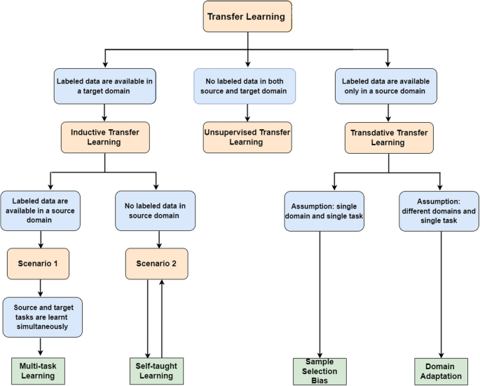

  

  Transfer learning strategies

  The following describes TL techniques categorized based on conventional DL algorithms:

  • 1. Inductive TL: target and source domains are similar, but differ in the task. The inductive bias of the source domain is applied by the algorithms to enhance the target task. Regardless of un- or classified data, the two categories of this approach are self-taught and multitask learning types [228].

  • 2. Unsupervised TL: similar to inductive TL, its focuses on unsupervised tasks in the target domain. The tasks differ despite similar target and source domains. Classified data are absent in both domains [229].

  • 3. Transudative TL: both target and source tasks are the same, but the domains differ. The source domain has many labeled data, but none in the target. The method is based on feature space or marginal probability [230].

  The listed transfer classifications denote three TL settings. The following approaches explain the transfer that revolves around the three TL categories:

  • 1. Instance transfer: an ideal idea is knowledge reuse from the source domain to the target task. Although the source domain cannot be directly reused, certain fractions may be reapplied with the target data to enhance output [231].

  • 2. Feature-representation transfer: error rates and domain divergence are minimized in this method by using good data representations from source to target domains. Based on the presence of classified data, un- or supervised techniques can be deployed for this type of transfer [232].

  • 3. Parameter transfer: in this transfer type, the models have similar parameters of prior hyper-parameter dissemination. Dissimilar from multitask learning (source & target tasks learned concurrently); extra weight-age is applied in TL for target domain loss to enhance performance [233].

  • 4. Relational-knowledge transfer: in this transfer type, dependent data with identical distribution is managed. This transfer is applicable for a data point related to another one, e.g., social network data [234].

• Types of deep transfer learning

  At times, it is difficult to distinguish TL from multitask learning and domain adaptation mainly because these methods attempt to resolve similar problems. Therefore, TL is reflective of a general concept that is applied to solve a task via task domain knowledge application.

  • 1. Domain adaptation

    In this domain, the marginal probability between target and source domains differs, e.g., $P(X_{s})\ne P(X_{t}))$. The integral shift in data dissemination of target and source domains needs alterations in learning transfer. For example, the corpus of movie reviews labeled negative or positive differs from that of product reviews—the classifier to train movie reviews will sense variation when classifying item reviews. Therefore, domain adaptation suits the TL approach in these examples [235,236,237,238,239].

  • 2. Domain confusion

    Besides highlighting the efficacy of feature-representation transfer, DL layers that capture feature sets can enhance transfer across domains and determine imminent domain-invariant aspects. It is crucial to ensure that both domain representations are near- or similar to enable effective learning. In order to do so, some pre-processing steps are required, as elaborated by Sun et al. in their paper [240], as well as Ganin et al. in [241]. Essentially, an additional goal is added to the source domain to ascertain similarity, thus causing domain confusion.

  • 3. Multitask learning

    In multitask learning, a number of tasks are learned concurrently without variance in source and target and one gains all data about the tasks at once. This differs from DL because one is clueless about the target task. Hence, multitask learning differs slightly from TL [242, 243].

  • 4. Zero-shot learning

    An extreme DL variant, zero-shot learning uses unclassified data for learning to make modifications at the training phase to exploit extra data so that hidden data can be comprehensible. In a book entitled Deep Learning, Goodfellow and co-authors discussed zero-shot learning based on three variables: conventional input and output variables (x & y, respectively), as well as a random variable that denotes the task (T). This model is trained to master conditional probability distribution; P(y|x, T). This learning type is suitable for machine translation, where the label is absent in the target language [244,245,246].

  • 5. One-shot learning

    As DL models need plenty of training data to learn weights, Deep Neural Networks (DNNs) are unsuitable. For example, a child exposed to an apple would be able to identify a variety of apples—but this is not the case for DL and ML approaches. A variant of TL, one-shot learning yields output with one training instance; thus suitable for actual settings with the absence of classified data for many scenarios (classification task) and for conditions that require the addition of new classes. In an article by Fei-Fei et al. [247], the term ‘one-shot learning’ was coined to describe a Bayesian framework variation that represents learning for the classification of objects. Since its emergence, this approach has been enhanced and applied in DL models [248].

  • 6. Few-shot learning

    This type involves training models to recognize new objects or classes with only a few examples, typically ranging from 1 to 10 examples per class. In other words, the goal of few-shot learning is to enable machines to learn quickly and efficiently with limited data. on the other hand, one-shot learning is a specific case of few-shot learning where the model is trained on only one instance per class. One-shot learning is considered a more challenging task than few-shot learning because the model must generalize well from a single instance, whereas few-shot learning allows for a small number of examples to be used for training. The challenges of interpreting multimodal time-series data from drone and quadruped robot platforms for remote sensing and photogrammetry have been discussed [249, 250], due to the expensive and time-consuming nature of data annotation in the training stage. The authors proposed a few-shot learning architecture based on a squeeze-and-attention structure that is computationally low-cost and accurate enough to meet certainty measures. The proposed architecture was tested on three datasets with multiple modalities and achieved competitive results. This study demonstrated the importance of developing robust algorithms for target detection in remote sensing applications, using limited training data.

• Transfer learning approaches

  The two TL methods are feature-extraction and fine-tuning [251,252,253].

  • 1. Feature-extraction

    Here, a well-trained CNN model is deployed to extract features for the target domain from a massive dataset, such as ImageNet. All completely connected layers in CNN models are discarded and all convolution layers are frozen. The latter layers are the feature extractor that adapts to new task. The extracted features are fed to the classifier form supervised ML or completely connected layers. lastly, only a new classifier is used to train, instead of the whole network, for the training process [254, 255].

  • 2. Fine-tuning

    This method is similar to feature extraction, except that the convolution layers of well-trained CNN are not frozen but their weights are updated during the training phase. Thus, the weight of convolution layers is initialized with CNN’s pre-trained weights when the classifier layers are initialized with random weights. Here, the whole system undergoes training [164, 256].

• Research problem in transfer learning for medical imaging

  One of the solutions to address the lack of training data is employing the pre-trained models of ImageNet for the target task. For some applications, this type of TL from ImageNet has significantly improved the results compared with training from scratch [257, 258]. However, for some other applications such as medical imaging applications, this type of TL from ImageNet does not help to address the issue of lack of training data. This is due to the mismatch in learned features between the natural image, e.g., ImageNet (color images), and medical images (gray-scale images such as MRI, CT, and X-ray) (see Fig. 8) [213, 259].

  Fig. 8

  

  Comparison between TL from ImageNet to nature images and medical images

  These models of ImageNet were designed to classify 1000 classes. However, medical images are ranging between 2 and 10 classes. Therefore, it results in the use of deeply heavy models.

  It has been proven that different domain of TL (such as ImageNet) does not significantly affect performance on medical imaging tasks, with lightweight models trained from scratch performing nearly as well as standard ImageNet models [260]. To end that, Alzubaidi, et al. proposed two different types of novel TL which effectively showed excellent results in several medical applications [23, 124]. One of the solutions was based on training the DL model on a big number of unlabelled images of a specific task then the model will be trained on a small, labeled dataset for that same task. This approach guarantees that the model will learn the relevant features and reduce the effort of the labeling process. It will offer the chance to use a shallow model with the desired input size. By using the same approach, several published articles have improved the effectiveness of these solutions for medical images and other domains [22, 123, 164, 261,262,263,264,265].

  Another solution was proposed by Azizi et al. [70] to improve the learned features of DL models by training them on a large number of unlabelled images of a specific task then the models will be trained on a small, labeled dataset for that same task.

  Figure 9 demonstrates the comparison of two models trained for the detection of shoulder abnormalities from our ongoing work. The first column is the original images with a red circle which is the region of interest marked by an expert. The second column is a model trained after TL from ImageNet while the third one is a model trained after TL from the same domain TL of the target dataset. As shown in the first row, both models correctly predicted the image based on their confidence values. However, the heatmap reveals that the first model is biased and inaccurate, failing to detect the region of interest indicated by the red circle. In contrast, the second model accurately identified the region of interest with a high confidence value. The second row illustrates that the first model missed the classification, while the second one correctly classified the sample. This example highlights the importance of the source of TL, as even a model with correct confidence values may not be trusted.

  Fig. 9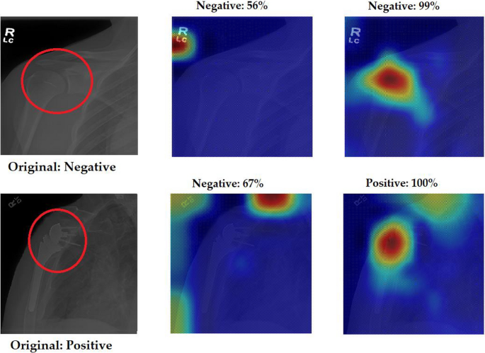

  

  Comparison between two different TL

• Instances of transfer learning for deep learning

  The TL has been applied in many areas within the DL field and real world applications, e.g., enhancing computer vision and NLP. The following describes some instances of TL used in DL.

  • 1. Transfer learning in NLP

    The capability of a system to analyze and comprehend human language (text/audio files) is NLP—to enhance human-system interaction. In fact, NLP is crucial for daily activities, including language contextualization tools, voice assistants, translations, speech recognition, and automated captions. Many DL models with NLP can be enhanced with TL, such as adding pre-trained layers that identify vocabulary or dialect and concurrent model training to identify language aspects. The method of TL can be used for model adaption across multiple languages. Models trained and refined in one language may be adapted for other similar languages. With vast English digitized resources, the models may be trained using a massive dataset before transferring the aspects to another language [266,267,268,269,270,271,272].

  • 2. Transfer learning in computer vision

    The capability of a system to make meaning from visual formats (images/videos) is known as computer vision. A massive volume of images is trained for DL models to reckon and group the images. Here, TL recycles elements of the computer vision algorithm for application in the new model. The accurate models generated via TL from training with massive data can be applied effectively for smaller image sets or even more general aspects (e.g., detecting object edges). Essentially, a specific model layer that detects objects/shapes can be trained. While refining and optimizing the model parameters, the TL sets the model functionality [273,274,275].

  • 3. Transfer learning in neural network

    The ANN is a crucial element in DL for simulating and replicating human brain functions. Notably, NN training usurps plenty of resources due to model intricacy. In fact, TL is crucial to minimize the use of resources and ascertain an efficient process. The development of new models includes the transfer of features or knowledge across networks. The use of knowledge in varied settings is a vital aspect of network building. Essentially, TL is typically limited to general tasks or processes that stay relevant in an assortment of scenarios [214, 215, 276].

  • 4. Transfer learning for Audio/Speech

    The DL model, similar to computer vision and NLP, can be applied to audio data. Models called Automatic Speech Recognition (ASR) formulated for the English language are broadly applied to enhance the performance of speech recognition in other languages. Another instance of TL application refers to automated speaker identification [177, 277, 278].

  There are more domains that used TL to address the issue of lack of training data as listed in Table 1.

  Table 1 Some examples of TL from the literature

• The future of transfer learning

  Widespread access to more powerful models formulated by conglomerates and related organizations dictate the future of DL models. It is crucial that the DL is adaptable and accessible to organizational demands and goals to revolutionize processes and businesses. However, only a handful of organizations possess the resources and expertise to train models and classify data. One challenge faced by supervised DL is obtaining a massive amount of classified data. Classifying countless data is labor-intensive and access to most data appears prohibitive to developing powerful models. With access to many classified data and resources, organizations can effectively develop algorithms. However, when used in other organizations, the model performance may differ due to environmental and training change impacts. Even the most accurate models would results in performance degradation in a different setting—a hindrance to DL when shifting to mainstream application. Imminently, TL has a significant function in resolving the said barrier. By integrating TL, the DL models can turn more powerful due to their ability to carry out specific tasks and settings. Hence, TL is denoted as an imminent driver for distributing DL models across new fields and areas.

Self-supervised learning

Self-supervised learning (SSL) is a technique of training DL models using large amounts of unannotated data and a small amount of annotated data, or using a pretext task to generate labels for the data. It is often used to pre-train models on large datasets and then fine-tune them on a smaller dataset with a different task in mind. SSL can be a useful solution for data scarcity, as it allows models to learn useful features from large amounts of unannotated data, which can then be fine-tuned on a smaller dataset for the target task [68,69,70,71].

One of the main benefits of SSL is that it allows models to learn useful features from large amounts of unannotated data, which can be useful in situations where annotated data is scarce or expensive to obtain. It can also be used to learn more robust and generalizable features, as the model is exposed to a larger variety of data during training [339, 340].

There are several types of SSL, including:

• Pretext tasks: these are tasks that are designed to generate labels for the data, which can then be utilized to train a DL model. Examples of pretext tasks include predicting the rotation of an image, predicting the next frame in a video, and predicting the mask for an image.

  One example of using a pretext task for SSL is the work done by Doersch et al. [341]. The authors trained a CNN to predict the relative location of randomly selected patches within an image. The CNN learned useful features from the images that could then be utilized for other tasks.

• Autoencoders: these are neural networks that are trained to reconstruct their input data. They are often utilized as a way to learn useful features from the data, which can then be utilized for other tasks.

  An example of using autoencoders for SSL is the work done by Masci et al. [342] where the authors trained a stacked autoencoder to learn features from images of faces. The learned features were then used to train a classifier to recognize the identities of the faces.

• Generative models: these models are trained to generate new data that is similar to the training data. Examples include Variational Autoencoders (VAEs) and Generative Adversarial Networks (GANs) which will be explained in the next section.

  An example of using generative models for SSL is the work done by Goodfellow et al. [343]. They trained a GAN to generate synthetic images that were similar to a dataset of real images. The generated images were used to train a classifier to recognize objects in real images.

• Contrastive learning: this SSL technique involves training a model to distinguish between different types of data. The model is then fine-tuned on a downstream task using the learned features.

  An example of using contrastive learning for SSL is the work done by He et al. [344] where they trained a CNN to distinguish between different types of images and used the learned features to train a classifier on a downstream task.

• Self-supervised multitask learning: this technique is based on training a single model on multiple tasks simultaneously, using a combination of supervised and unsupervised learning. The model learns to solve multiple tasks using the shared features learned from the unsupervised tasks.

  An example of using self-supervised multitask learning is the work done by Caruana et al. [345]. The authors trained a single neural network to perform multiple tasks simultaneously, using both supervised and unsupervised learning. The network learned to solve the tasks using the shared features learned from the unsupervised tasks.

Generative adversarial networks (GANs)

The GANs are regarded as a type of DL network that yields data with similar features as the input real data. Via GANs, representations are learned without intricate training datasets, as learning denotes regaining proportional signals based on a paired-network competitive process. Representations that GANs learn can be applied in, for example, image synthesis, classification, and super-resolution; style transfer; and editing of semantic image [346, 347]. The GANs overcome insufficient training data. Goodfellow et al. [348] initiated the adversarial method for learning GAN models. The GAN is a game denoting min-max, two-person, and zero-sum (the loss of one player is an advantage of another). The GAN consists of the generator (G) and discriminator (D). The G deceives another player by faking sample dissemination, while D distinguishes real from fake samples. A sample is more likely to be real if the probability value is higher (0 = fake sample, 0.5 = optimal solution). Upon nearing an optimal solution, D would not be able to distinguish real from fake samples [349,350,351,352]. Figure 10 illustrates the general GAN architecture.

Fig. 10

The general GAN architecture

• 1. Generator (G): a network that yields images using random noise Z, G(z). Gaussian noise is typically selected as the input—a random point in latent space. Iterative updates are made to parameters of G and D while GAN training.

• 2. Discriminator (D): this network ascertains if an image is a real or fake distribution. Upon receiving input image X, it generates output D(x); signifying X is probably not fake. Output = 1 denotes the distribution of the real image, while D = 0 signifies otherwise.

• Variants of GAN

  Enhancements made to GAN architecture (Fig. 11) are explained in the following:

  Fig. 11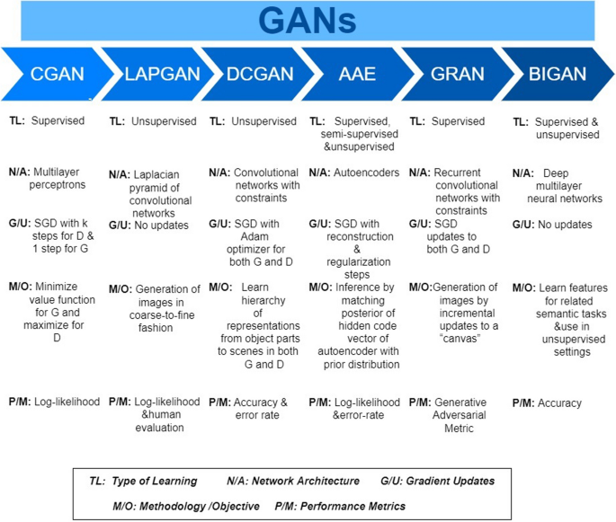

  

  Variants of GAN

  • 1. Fully connected GANs

    The initial GAN MA had full NN connections for D and G [348]. This MA was applied for the detection of simple images, e.g., the Toronto Face dataset (TFD), MNIST, and CIFAR10 (natural images).

  • 2. Conditional GANs (CGAN)

    Upon extension, D and G networks are conditioned on additional data (y) to overcome reliance on random variables in the original model [353]. y denotes auxiliary data from other modalities or class labels. Conditional data are used by feeding y into G and D networks as an extra input layer (see Fig. 12). In the G network, prior input noise pz(z) and y are integrated in joint hidden representation, while the adversarial training framework permits considerable flexibility in the composition of this hidden representation [353]. In the D network, both x and y are presented as inputs to a D function.

    Fig. 12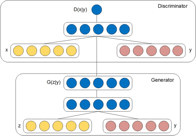

    

    Conditional GAN’s architecture

  • 3. Laplacian pyramid of adversarial network (LAPGAN)

    Using a cascade of convolutional networks with the LAPGAN model, Denton et al. [354] introduced image generation in a coarse to fine manner. Hence, a multiscale structure of natural images could be exploited to build GAN models by taking a certain level of image structure based on LAPGAN. Built from the Gaussian pyramid, the Laplacian pyramid uses these functions: downsampling d(.) and upsampling u(.). Let G(I) = $[I_{0};I_{1}; \ldots ; I_{K}]$be Gaussian pyramid, where $I_{0}$ = I while $I_{k}$ denotes repeated k of d(.) to I. Laplacian pyramid’s coefficient $h_{k}$ (level k) signifies the variance among adjacent levels within the Gaussian pyramid, in which unsampling has a smaller value with u(.) (Eq. 3).

    $$h_{k}=L_{k}(I) = G_{k}(I)- u(G_{k+1}(I))= I_{k}-u(I_{k+1})$$

    (3)

    Coefficients of Laplacian pyramid $[h_{1}; \ldots ; h_{k}]$ is reconstructed via backward recurrence, as in Eq. (4):

    $$I_{k}=u(I_{k+1}+h_{k})$$

    (4)

    Convolutional generative models, which are needed to train LAPGAN, capture coefficients $h_{k}$ distribution for varied Laplacian pyramid levels. These generative models, during reconstruction, yield $h_{k}$. Hence, the modification that takes place in Eq. (4) is expressed in Eq. (5):

    $$\bar{I_{k}}=u((\bar{I_{k-1}})+\bar{h_{k}})= u(\bar{I_{k-1}})+ G_{k}(z_{k}, u(\bar{I_{k-1}}))$$

    (5)

    Training image I is used to constructing the Laplacian pyramid. The stochastic choice is made at every level for coefficient $h_{k}$ construction via $G_{k}$ generation or via the standard procedure. The CGAN model is used by LAPGAN by incorporating low = pass image $\imath _{k}$ to both G and D. The LAPGAN performance was assessed using three datasets: LSUN, CIFAR10, and STL10. The assessment was conducted through the comparisons of human sample examination, log-likelihood, and generated image sample quality.

  • 4. Deep convolutional GAN (DCGAN)

    A new class of CNN was initiated by Radford et al. [355] called DCGANs that can resolve the following architectural issues noted in CNN MA:

    • Hidden layers that are completely connected are discarded, while pooling layers are substituted with fractional- and stridden convolutions on G and D, respectively.

    • Batch normalization is applied for both G and D models.

    • ReLU and LeakyReLU activation is used in G (except the final layer) and D layers, respectively.

    The G in DCGAN used in LSUN sample scene modeling is portrayed in Fig. 13. Its performance was compared with that of SVHN, LSUN, CIFAR10, and Imagnet 1K datasets. First, DCGAN was used as a feature extractor to determine the quality of unsupervised representation learning, followed by the determination of accuracy performance by fitting a linear model above the features. Notably, G displayed the ability to disregard some elements of the scene, e.g., furniture and windows. Good outcomes were noted when vector arithmetic was executed on face samples.

    Fig. 13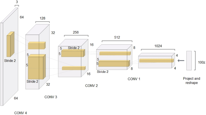

    

    DCGAN’s architecture

  • 5. Adversarial autoencoders (AAE)

    The AAE, which was proposed by Makhzani et al. [356], refers to a probabilistic autoencoder that applies GAN to carry out variational inference. This is done by matching arbitrary prior dissemination with aggregated posterior of hidden code vector in autoencoder. The autoencoder in AAE undergoes training with two aims—criteria for conventional reconstruction error and adversarial training. Next, conversion of the data distribution to the prior one is learned by the encoder at post-training. The decoder, on the other hand, learns the deep generative model that portrays that prior to data distribution (Fig. 14). The MA of AAE is given below: Where x and z are the input and latent code vectors of autoencoder. p(z), q(z|x), and p(x|z) reflect imposed prior, encoding, and decoding distributions, respectively. Next, pd(x) and p(x) signify data and model distributions, respectively. The aggregated posterior distribution of q(z) on hidden code vector of the autoencoder is defined as q(z|x) (autoencoder encoding function), as expressed in Eq. (6):

    $$q(z)=\int _{x}q(z|x)p_{d}(x)dx$$

    (6)

    Regularisation of autoencoder in AAE is performed by matching arbitrary prior p(z) with aggregated posterior q(z). The adversarial G network serves as an encoder for autoencoder q(z|x)). Both autoencoder and adversarial networks are jointly trained with gradient descent in reconstruction and regularisation stages. Both the encoder and decoder are updated by the autoencoder in the reconstruction stage to minimize input glitches. The D is updated by an adversarial network in the regularisation stage to distinguish true samples from fake ones, and followed by a generative model update to confuse D. During the adversarial training, AAE includes labels as well to offer a better distribution shape for hidden code. Single-hot vector, which is included in discriminative network input to link distribution mode with the label, is a switch that chooses a decision boundary based on a class label for a discriminative network. The vector has an extra class related to unclassified data. This extra class functions when unclassified data are found so that the decision boundary can be chosen for full Gaussian distribution.

    Fig. 14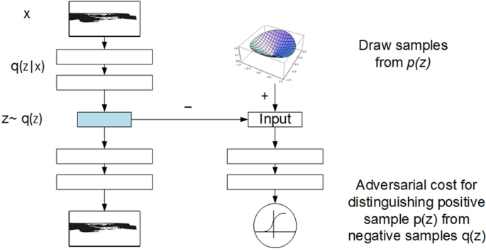

    

    AAE’s architecture

  • 6. Generative recurrent adversarial networks (GRAN)

    The GRAN, introduced by Im et al. [357], has recurrent computation, produced from unrolled optimization based on gradient, which incrementally develops images for visual canvas (see Fig. 15). Current canvas images are extracted from a convolutional network encoder. The decoder is fed with generated and reference image codes to decide on canvas updates. Functions f and g are GRAN decoder and encoder, respectively. The G in GRAN has a recurrent feedback loop, which receives noise samples sequence from $z \sim p(z)$ prior distribution, to draw results for varied time steps; $C_{1}$; $C_{2}; \ldots ;$$C_{T}$ Sample z from prior distribution is moved to function f(.) at time step (t) with hidden state $h_{c,t}$, where $h_{c,t}$ is the current encoded status of past Ct − 1 drawing. Ct denotes that drawn at time t on canvas with function f(.) output. Function g(.) mimics function f(.) in inverse. Gathering samples at every time step produces the last sample drawn on canvas, C. Function f(.) is the decoder that accepts noise sample z and past hidden state input $h_{c,t}$, while function g(.) is the encoder that offers output $C_{t-1}$ hidden representation for time step t. Dissimilar to the rest, GRAN begins with the decoder.

    Fig. 15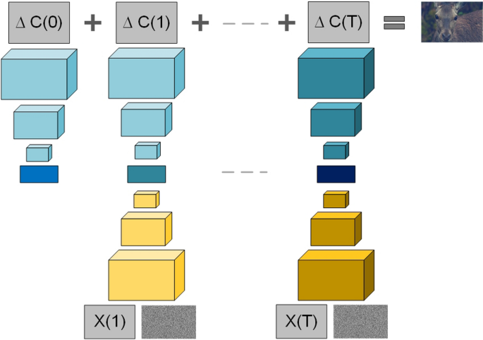

    

    GRAN’s architecture

  • 7. Bidirectional GAN (BiGAN)

    The BiGAN (see Fig. 16) was proposed by Donahue et al. [358] to learn data distribution inverse mapping and semantics, in which the learned feature representations are re-projected into latent space. Referring to Fig. 9, apart from G deriving from GAN, BiGAN has an encoder E that maps data x to latent representation z. The BiGAN D discriminates not only in data space [x versus G(z)] but jointly in data and latent spaces [tuples (x;E(x)) versus (G(z); z)], where the latent component is encoder output E(x) or G input z. Based on GAN targets, BiGAN encoder E can learn to invert G.

    Fig. 16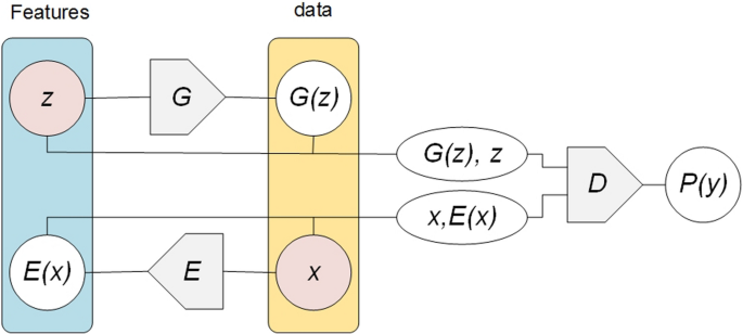

    

    BiGAN’s architecture

• GAN applications

  The GAN yields real-like samples with arbitrary latent vector z, thus dismissing the identification of the real distribution of data. Thus, GAN has been used in many academic and engineering fields. This section presents the applications of GANs in terms of generating new data to enhance training set [359,360,361].

  • 1. Generation of high-quality images

    Recent studies on GAN have enhanced both the usability and quality of image production abilities, such as the LAPGAN model [354] discussed Before. Several publications have addressed the issue of lack of training data using GANs [350, 362,363,364].

    The Self-Attention GAN (SAGAN) was initiated by Zhang et al. [365] to enable long-range, attention-driven reliance modeling that produces images. This is dissimilar from convolutional GAN, which yields details with high resolution for spatially local points within feature maps with low resolution. The SAGAN, which adds cues-generating details from all feature areas, yields excellent outcomes that lowered Frechet Inception Distance (FID) to 18.65 from 27.62 and hiked Inception Score (IS) to 52.52 from 36.8 for the ImageNet dataset.

    The BigGans was introduced by Brock et al. [366] to yield diverse and high-resolution samples from intricate datasets (ImageNet) by using the largest scale to train GAN. Orthogonal regularisation was used for G to make a ‘truncation trick’ that enables the control of trade-off between sample variety and fidelity by minimizing G input variance. Further alteration enabled the model to synthesize class-conditional images. The model, upon being trained using ImageNet (resolution: 128 $\times$ 128), scored 166.5 and 7.4 for IS and FID, respectively; which was better than the model described above.

    A G network for GAN was initiated in light of style transfer [367, 368]. The model displayed several noteworthy outcomes: enabled scale-specific and intuitive synthesis control, automatic learning, stochastic difference noted in the produced images (e.g., hair & freckles), and unsupervised segregation of attributed with high level (identity & pose if trained using human faces). Meanwhile, Huang et al. [369] introduced GANs that operated on intermediate representations and not images with low resolution. This model is similar to LAPGAN with extended CGAN as D and G networks could accept extra labeled data as input—a popular method to date that enhances image quality. In another instance, Reed et al. [370] applied GAN for image synthesis from texts (reverse captioning). To describe, a trained GAN may produce images that match certain descriptions, such as that of the following text: white with some black on its head and wings and a long orange beak. Along with texts, image location can be conditioned using a Generative Adversarial What-Where Network (GAWWN) that incrementally builds big images with the support of an interactive interface and bounding box supplied by user [371]. As for CGAN, besides synthesizing new samples with certain features, it permits users to create tools to edit images [372].

    For maximizing one/many neurons activation in a segregated classifier network, Nguyen et al. [373] introduced a novel approach that performs new image synthesis via gradient ascent in the latent space of the G network. The extension of this method incorporated extra prior on latent code, which enhanced sample diversity and quality—yielding high-quality images (resolution: 227 $\times$ 227) for all ImageNet data [374]. Additionally, Plug and Play Generative Networks (PPGNs) were introduced possessing (1) G network that draws multiple image types and (2) a substitutable condition network that informs what G should draw. As a result, the images were conditioned on the caption (C = image captioning network) and class (C = ImageNet/MIT Places classification network).

    Next, the GAN model was used by Salimans et al. [375] to execute training with novel features based on two aspects: semi-supervised learning and the production of visually-realistic human images. This model yielded accurate outputs using semi-supervised classification on SVHN, MNIST, and CIFAR10. Based on the Turing test, the produced images were verified of having high quality. While the CIFAR10 samples displayed a 21.3% human error rate, those of MNIST were near-similar to real data.

    Wasserstein GAN (WGAN) was used by Huang et al. [376] for density reconstruction in dynamic topography. Wasserstein GAN was proposed by Arjovsky et al. [377] to enable stable training but ended up failing to converge and producing poor samples. These issues, according to Gulrajani et al. [378], were due to clipping weight to apply the Lipschitz constraint on the critic. Alternative clipping weights were, thus, used to penalize the norm of critic gradient based on input. This resulted in better training for multiple GAN MAs with nearly nil hyperparameter tuning, inclusive of language models with continuous G and 101-layer ResNets, as well as high-quality yields on LSUN and CIFAR10. Based on what was discussed above, we believe GAN is an effective solution to generate more data to address both lack of data and imbalanced data [359,360,361, 379, 380].

  • 2. Image inpainting

    Missing parts reconstruction in images, or image inpainting, makes the reconstructed areas undetectable. Hence, damaged areas are restored and undesired objects are discarded in images. GANs have been applied to address this issue [381,382,383,384].

    The recent DL approaches have the ability to solve missing parts in images via the image inpainting technique, thus yielding perfect image textures and structures. Inferring arbitrary huge missing image parts via image semantics is called ‘semantic inpainting’ [385, 386]. The demand for high-level context prediction poses more difficulty in this method when compared to image completion or past inpainting methods that eliminate whole objects and address inauthentic data corruption.

    A method based on a deep generative model was initiated by Yu et al. [387] to apply surrounding image characteristics and synthesize image structures for better prediction. This CNN feed-forward model process varied-sizes and multi-hole images at random areas during the testing phase. Experimental work involving natural images (Places 2 & ImageNet), textures (DTD), and face samples (CelebA & HQ) revealed that the introduced model yielded higher-quality inpainting outcomes. Another study introduced an inpainting system in the DL model to complete images using inputs and free-form masks [388]. Using gated convolutions, the system learned millions of unlabelled images to address vanilla convolution problems (generalized partial convolution & input pixels being valid) by offering a mechanism to learn dynamic features for channels across all layers at each spatial region.

    A GAN loss model (SN-Patch GAN) using D with normalized spectral on patches of dense images [388] is rapid, non-intricate, and offers stable training. The extended version and automatic image inpainting revealed more flexible and higher-quality yields. Using edge G and followed by an image completion system, Nazeri et al. [389] built a model with a double-stage adversary. Missing region edges in images are hallucinated by edge G, and these edges are filled via the image completion system as a priori. The model was assessed using Paris Street View, CelebA, and Places2 datasets.

    A new semantic image inpainting model was proposed by Yeh et al. [390] based on GAN MA, whereby semantic inpainting was viewed as an issue of image generation. Their adversarial model [391, 392] had been trained to seek encoding of corrupted image ‘closest’ to the target image in latent space. Next, the image is reconstructed using G via encoding. ‘Closest’ is the loss of weighted context in the corrupted image and unrealistic images penalized via prior loss. In comparison to CE, this approach dismisses masks for training and can be applied for randomly-structured missing areas at the inference phase. This technique was assessed with CUB-Birds [393], CelebA [394], and SVHN [395] datasets with varied missing areas. The method gave more realistic images than other approaches.

  • 3. Super-resolution

    Upscaling images or videos require super-resolution, as it upgrades low-resolution images to high resolution by incorporating realistic image details at the training phase [396,397,398]. For instance, a new training approach was initiated by Karras et al. [399] to progressively grow G and D; begin at low resolution, and new layers are increasingly included to model fine details during training. This approach offer better speed and stability while training, thus generating high-quality images using CelebA.

    The extension of prior models, the SRGAN approach [400], is embedded with an adversarial loss element that constrains images to stay on the manifold of natural images. Imminently, the G in SRGAN holds low-resolution images and infers natural realistic images with a four-time scaling factor. Adversarial loss, dissimilar from other GAN models, is an aspect of the larger loss function that incorporates permanent loss from a pre-trained classifier, as well as regularisation loss that yields images that are spatially coherent. The entire solution is constrained by adversarial loss to manifold natural images, thus generating better solutions. Access to curated training data is a hindrance to DL model customization. Nonetheless, SRGAN customizes specific domains in a straightaway manner because new training image pairs are constructed easily by down-sampling high-resolution image corpus. Essentially, the image domain in the training set dictates the yield of GAN with realistic details.

    To improve SRGAN visual quality, Wang et al. [401] assessed the following three elements: perpetual loss, network architecture, and adversarial loss—the initiation of Enhance SRGAN (ESRGAN). The fundamental network building unit is composed of Residual-in-Residual Dense Block (RRDB) in the absence of batch normalization. The very idea derived from relativistic GAN, which enables D to predict, rather than absolute value, but corresponding realness. To gain stronger supervision for texture recovery and brightness consistency, the perpetual loss was enhanced with features prior to activation. The ESRGAN gave higher visual quality with more natural and realistic texture than SRGAN—champion in PIRM2018-SR Challenge (region 3; the best perceptual index).

    As many techniques end up yielding low-quality and low-resolution images in real scenarios, Bulat et al. [402] introduced a two-stage process: (1) High-to-Low GAN is trained to learn down-sampling and degrading images with high-resolution, and (2) the network output is applied to train Low-to-High GAN in order to generate images with super-resolution.

  • 4. Video prediction and generation

    An issue in computer vision is comprehending scene dynamics and object motion. A model is needed for scene transformation in video generation (prediction of the future) and recognition (grouping of actions). Building this model is, however, not easy due to motion in scenes and objects [403, 404]. A GAN for the video was proposed by Vondrick et al. [405] to untangle the scene foreground from the background via spatiotemporal convolutional architecture. In predicting the future of static images, the proposed model could produce a 1-s short video at a complete frame rate, which is better than a simple baseline. Further assessment revealed that the model could learn features to reckon actions at minimum supervision—scene dynamics are viable for representation learning. Several works were proposed for same purpose using GANs [404, 406, 407]

    The Motion and Content decomposed GAN (MoCoGAN) was introduced by Tulyakov et al. [408] to yield videos. Videos are made by generating a sequence of random vectors [with content (fixed) & motion (stochastic) parts)] to that of video frames. Using video and image Ds, a new adversarial learning mechanism was devised to learn content and motion decomposition unsupervised. The model efficacy was verified empirically via quantitative and qualitative approaches. This approach has been improved in different ways [360, 404, 407].

  • 5. Anime character generation

    Apart from requiring experts for routine tasks, animation production and game development are costly. Anime characters can be colorized and auto-generated using GAN [409,410,411,412,413]. These G and D have multiple ReLU with skip connections, convolutional layers, and batch normalization. The CartoonGAN, a solution that transforms real-world photos into cartoons was initiated by Chen et al. [414] for computer graphics and computer vision applications. The easy training phase involves cartoon images and unpaired photos. The two losses for cartoon styling are (1) semantic content loss (sparse regularisation for high-level feature maps of VGG network to cope with photo-cartoon style variation) and (2) edge-promoting adversarial loss (preserves clear edges). To automatically generate anime characters, Jin et al. [411] combined GAN training methods and a clean dataset to yield realistic facial images. The SRResNet was modified to a G model (see Fig. 17) that applies 3 subpixel CNN (to upscale the feature map) and has 16 Res-Blocks. The architecture of D displayed in Fig. 17 has 10 Res-Blocks. Due to correlations in mini-batch that lead to unwanted gradient norm calculation, layers of batch normalization were discarded from D. Additional completely connected layers were added to the final convolution layer as the classifier of the attribute. Weights initialized from Gaussian distribution had 0:02 and 0 standard deviation and mean values. Figure 18 portrays an anime character generated by GAN.

    Fig. 17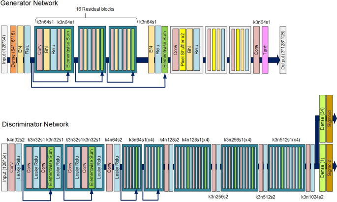

    

    The architecture of Anime G & D

    Fig. 18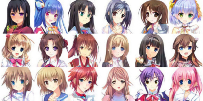

    

    Anime samples generated by GANs

  • 6. Image-to-image translation

    The translation of input to output images can be performed using CGAN—a recurring theme in computer vision, computer graphics, and image processing. This pix2pix model resolves these image-related issues [415,416,417]. Additionally, a loss function may be devised using the pix2pix model in order to train input-to-output image mapping. It yields exceptional outcomes for varied computer vision problems that demanded black-white image colorization, semantic segmentation, attaining maps from aerial photos, and segregated machines [415].

    The model was extended to produce CycleGAN [418] by embedding cycle consistency loss that preserves the original image after translation and reverse translation cycle. As paired images are eliminated from the training phase, the data preparation process becomes simpler and is open to other multiple approaches. The artistic style transfer [419], for example, gives a natural image with Monet or Picasso style by training using natural images and unpaired paintings. Novel samples that match the training set can be achieved by GAN, along with style transfer (modifies image visual style), domain adaptation (the generality of new domains with unclassified data in the target domain), and the latest, TL (import of existing knowledge to simplify learning) approaches [420]. Nonetheless, the general analogy synthesis issue is untapped. Hence, Taigman et al. [420] overcame this problem by separating labeled samples from domains T and S, as well as by incorporating a multivariate function (f) for mapping; $G: S \rightarrow T$ such that $f(x) \sim f(G(x))$. The DNNs of a certain structure were applied, where G denotes learning (g) and input (f) functions composition. The compound loss that integrates multiple terms was deployed as well. The proposed technique can visual domains (face images and digits) and generate realistic new images from unseen samples, while concurrently retaining identities.

    A generative network was segregated into two by Chen et al. [421] so that each looks into a subtask alone. The attention network estimated spatial attention maps of images, while the transformation network translated objects. The attention map produced in the initial step is sparse to enable more attention placed on the target object and should remain constant regardless of transfiguration. More instructions are given while learning the attention network due to image segmentation. The outcomes revealed the importance of assessing attention during the transfiguration, whereby the algorithm introduced can learn precise attention to enhance the quality of the produced images.

    In the Multimodal Unsupervised Image-to-image Translation (MUNIT) model introduced by Huang et al. [422], image representation is decomposed into a content mode (domain-invariant) and style code (detects domain-specific attributes). The translation of an image to another domain involves the recombination of content code with random style code deriving from the target domain. Upon comparing the proposed model with other current models, the latter displayed more benefits.

    The Exemplar Guided and Semantically Consistent Image-to-image Translation (EGSC-IT) network introduced by Ma et al. [423] can be applied to perform the translation process on samples in the target domain. An image consists of a shared content aspect (shared across domains) and a style aspect (specific to the domain). The Adaptive Instance Normalisation applies the shared content aspect to enable style information transfer from the target domain to the source domain. The concept of the feature was deployed to hinder semantic inconsistency while translation (due to variations of the large inner and cross-domain) and to offer a coarse semantic guide in the absence of a semantic label. The Single GAN was introduced by Yu et al. [424] to execute multi-domain image-to-image translation with single G. In order to ascertain A domain code was deployed to integrate multiple optimization goals and to control varied generative activities. The results for unclassified data revealed superior performance by the proposed model when translating between the two domains. CycleGAN has been used in several applications such as medical imaging and plant diseases to address the issue of imbalanced datasets [425,426,427,428]. Figure 19 shows an example of CycleGAN with CT images.

    Fig. 19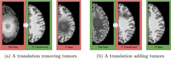

    

    An example of medical image translation [429]

  • 7. Text-to-image translation

    One of the impressive applications of GANs is text-to-image translation [430,431,432,433]. Using GAN, Fedus et al. [434] enhanced sample quality by explicitly training G to yield high-quality samples that displayed successful image production. The actor-critic CGAN can complete missing text conditioned on the context. Evidently, this gave more realistic un- and conditional text samples quantitatively and qualitatively, in comparison to maximum likelihood trained model.

    With the benefits of automatic synthesis of realistic images from text, Denton et al. [354] applied the Laplacian pyramid with adversarial G and D to synthesize images at many resolutions. Images with high resolution that can condition on class labels were produced with control. Using a standard convolutional decoder, Radford et al. [355] built a stable and effective MA by including batch normalization to attain exceptional image synthesis outcomes.

    The GAWWN was used by Reed et al. [370] to synthesize images from text descriptions (reverse captioning). Besides conditioning on image location [371], the model supports an interactive interface that increasingly builds up big images with textual descriptions and bounding boxes supplied by the user. As for CGANs, it synthesizes new samples with certain features and enables the development of tools to intuitively edit images, such as hairstyle editing or giving a younger look in images [435]. Figure 20 shows an example of text-to-image translation.

    Fig. 20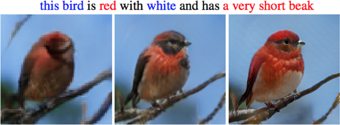

    

    An example of text-to-image translation [436]

  • 8. Face aging

    Progression and regression of face age (or face rejuvenation and aging) render face images regardless of aging effect, while simultaneously preserving personalized face features (i.e., personality) [437,438,439,440]. A conditional AAE (CAAE) was initiated by Zhang et al. [441] to learn face manifold. The control of age attribute assures flexibility to gain regression and progression concurrently. Some advantages of CAAE are: (1) gains age regression and progression to produce realistic face images, (2) dismissal of paired samples while training and labeled face while testing—ascertaining model generality and flexibility, (3) disentangled personality and age in latent vector space preserve personality and hinder ghosting artifacts, as well as (4) robust against occlusion, pose, and expression variations as CAAE imposes D on the encoder and G. The D on the encoder and G offer smooth transition in latent space and realistic face images, respectively. Thus, CAAE yields images with higher quality than AAE. The CAAE had been assessed with CACD [442] and Morph [443] datasets.

    A synthetic aging method was initiated by Antipov et al. [444] for human faces using Age CGAN (Age-cGAN), comprising of dual steps: (1) input face reconstruction that demands optimization problem resolution to seek optimal latent approximation, (2) and face aging executed via simple conditions change at G input. This approach introduces ‘Identity-Preserving’ latent vector optimization that preserves the original identity during the reconstruction phase, besides modifying other facial features. Figure 21 shows an example of face age.

    Fig. 21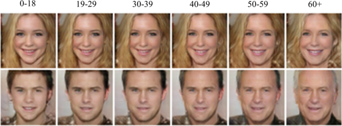

    

    An example of face age [444]

  • 9. Image blending

    Mixing of two images is called ‘image blending’, where the output image is combined with input images pixel values and GANs showed an excellent performance [445].

    The dense image matching method was initiated by Gracias et al. [446] to enable copy and paste of only the related pixels. Significant variances between source images dismiss the model usage. One way is by making a smooth transition to hide artifacts in composited images.

    The Gaussian–Poisson GAN (GP-GAN), which was introduced by Wu et al. [447], combines the strengths of GANs and approaches based on a classical gradient—The initial study that assessed GAN ability in high-resolution image blending task. The Gaussian–Poisson Equation was developed to address the high-resolution image blending issue—a joint optimization constrained by color and gradient data. Color data are obtained from Blending GAN, which was introduced to learn the mapping between well-blended and composited images; while gradient data are generated from gradient filters. Apart from producing realistic and high-resolution images, the proposed model generated less undesired artifacts and bleeding. The experimental outcomes verified the superior performance of the proposed model over other models using Transient Attributes dataset.

Model architecture

There are some solutions that help to deal with small datasets related to MA. These solutions can help when it is impossible to collect or generate more training data.

• 1. Model complexity

  Reducing model complexity DL due to limited datasets can help avoid overfitting and improve generalization to new, unseen data. This can be achieved by reducing the number of layers or nodes in the model, adopting simpler activation functions, or regularisation techniques. While reducing model complexity can mitigate the risk of overfitting, it may also limit the model’s capacity to represent complex relationships in the data, resulting in underfitting and lower accuracy. Furthermore, reducing model complexity may limit the model’s ability to learn from high-dimensional data, which can lead to poorer performance in tasks such as medical images or speech recognition. Therefore, it is crucial to carefully balance the trade-offs between model complexity and model performance on both the training and test data [448,449,450,451].

  Brigato et al. [452] performed a wide variety of experiments with varied DL MAs on datasets of limited size. Model intricacy should not be undermined when only a few samples are available in a class. Opposed to the literature, the authors revealed that certain current models may be improved in several configurations by using models with low intricacy. Non-intricate CNNs can perform better than the current MAs without augmentation of data and with inadequate training data. They added recognition performance may be improved by massive margins with standard data augmentation. This signifies the importance of devising complex data augmentation and generation models in case of limited data. Lastly, they reported that dropout—a broadly applied regularisation method—maintains its role despite data scarcity. Their findings were empirically validated with sub-sampled CIFAR10, Fashion-MNIST, and SVHN benchmarks.

• 2. Loss functions

  Loss functions are an essential component of DL models, as they are used to measure the difference between predicted and actual values. In the case of data scarcity, selecting an appropriate loss function becomes critical as the model needs to be trained with limited data samples. Therefore, it is essential to analyze and evaluate different loss functions that can help address the data scarcity problem. Some of the commonly used ones are:

  • Mean Squared Error (MSE) is a popular loss function used in DL for regression problems. It measures the average squared difference between predicted and actual values [453].

  • Mean Absolute Error (MAE) measures the average absolute difference between predicted and actual values [454]. This function is also known for regression problems.

  • Cross-Entropy Loss is known for use of multi-class classification problems. It measures the dissimilarity between the predicted probability distribution and the actual probability distribution of the target variable [455]. It is commonly used in tasks such as image classification and natural language processing.

  • Hinge Loss is commonly used for binary classification problems where is commonly used in support vector machines (SVMs). It encourages correct classification by penalizing incorrect predictions linearly [456].

  • Focal Loss is well-known for imbalanced classification problems. It is designed to give more weight to hard-to-classify examples, reducing the impact of easy-to-classify examples and improving performance on the minority class. It is commonly used in object detection and segmentation tasks [457].

  • Triplet Loss is used for learning representations in siamese networks or other similar architectures. It measures the distance between anchor, positive, and negative samples [458].

  • Contrastive Loss is used to learn the similarity between two inputs, and it penalizes the model for dissimilar inputs and rewards the model for similar inputs [459].

  • Sparsemax Loss is a probabilistic activation function that can be used in classification tasks [460]. It encourages the model to assign low probabilities to irrelevant classes.

  • Kullback–Leibler (KL) Divergence Loss is used for measuring the difference between two probability distributions [453]. It is often used in generative models, such as Variational Autoencoders (VAEs).

  • Huber Loss is used in regression tasks and provides a combination of Mean Absolute Error (MAE) and Mean Squared Error (MSE) loss functions [461].

  • Quantile Loss is known for quantile regression problems. It measures the difference between the predicted quantile and the actual value at that quantile, with a different loss function for each quantile. It is commonly used in financial forecasting and risk analysis [462].

  • Center Loss is used for face recognition tasks and minimizes the distance between the features extracted by the DL model and their corresponding class centers [463].

  • Wing Loss is designed to be robust to outliers by penalizing large errors less than Mean Squared Error (MSE) Loss [464]. It is commonly used in tasks such as facial landmark detection and human pose estimation.

  • Cosine Loss is used to optimize the cosine similarity between two feature vectors in a high-dimensional space. It is commonly used in tasks such as face recognition and image retrieval [465].

  In evaluating the performance of loss functions on the data scarcity problem, we can consider metrics such as accuracy, precision, recall, F1 score, and area under the curve (AUC). These metrics provide a comprehensive evaluation of the performance of the model in addressing the data scarcity problem. By comparing the performance of different loss functions on these metrics, we can determine which loss function is most effective in improving the model’s performance when training data is limited.

  In terms of processing time, different loss functions have different computational requirements. For instance, mean squared error and mean absolute error are computationally less expensive than cross-entropy and hinge loss. However, this difference in computational cost may be insignificant in practice, especially with the use of modern GPUs that can handle complex computations with ease. There are several challenges associated with selecting and using loss functions in deep learning. It can be challenging to choose the right loss function for a specific problem, especially when the data is scarce. Different loss functions have different strengths and weaknesses, and the wrong choice can lead to suboptimal results, some of which are:

  • Imbalanced datasets mean one class has significantly fewer samples than the others. It can be challenging to find a loss function that balances the trade-off between correctly identifying the minority class while not misclassifying the majority class too often.

  • Noisy data can be a challenge when selecting an appropriate loss function. Noisy data can cause the model to learn incorrect patterns, leading to poor performance.

  • Overfitting is an issue when some loss functions are prone to it, especially when the model is too complex or when the data is scarce. Overfitting occurs when the model learns to fit the training data too well, resulting in poor performance on the test data.

  • Optimization challenges can appear in some loss functions that can be difficult to optimize. This can lead to slow convergence or getting stuck in local minima.

  • Model interpretability can be an issue when some loss functions are more difficult to interpret than others which making it harder to understand why the model makes certain predictions.

  In summary, selecting an appropriate loss function is critical in addressing the data scarcity problem in DL. Evaluating the performance of different loss functions using relevant metrics provides a comprehensive understanding of their effectiveness in improving model performance. While some loss functions may require more computational resources than others, this difference may be insignificant in practice, given the availability of modern computing infrastructure.

• 3. Ensemble classifiers

  Ensemble classifiers are a powerful technique for addressing the problem of limited training datasets in DL. By combining the predictions of multiple models trained on different subsets of data or with different algorithms, ensemble classifiers can improve the overall accuracy, robustness, and generalisability of the model. Additionally, ensemble classifiers can help to reduce the risk of overfitting and identify and correct biases that may exist in any single model, making them a valuable tool for improving the reliability and accuracy of DL models in situations where training data is limited [14, 466, 467].

  Olson et al. [153] depicted that DNNs can generalize well on small, noisy datasets despite memorizing the training data. To explain this behavior, the authors developed a novel perspective on NNs by viewing them through the lens of ensemble classifiers. When training NNs, it is important to choose an architecture that allows adequate capacity to fit the training data, and later, re-scale with regularisation [468]. On the contrary, the random forest holds that training data can perfectly fit very deep decision trees, and then, rely on randomization and averaging for variance reduction. This notion can be applied to DNN. Instead of each layer presenting an ever-increasing hierarchy of features, it is plausible that the final layers offer an ensemble mechanism. Finally, they reported that small datasets and relatively small network sizes have computational advantages, which allow for rapid experimentation. Some recent studies explained NN generalization as intractable on networks with millions of parameters: Schatten norms, for instance, require computing full SVD [469]. In the study context, such calculations are trivial. Thus, future studies should discern a mechanism for decorrelation, as well as assess the link between decorrelation and generalization.

Physics-informed neural network (PINN)

Physics-Informed Neural Network (PINN) is another DL technique that can cope with problems with insufficient data or even without labeled data [470,471,472,473]. Apart from using pure data, PINNs can also integrate physics laws to train neural networks for unknown systems [474]. We note that the physics laws can be equations that are derived from conservation principles or empirical models that are summarized by calibrations of observations. Such as the Navier–Stokes equations for fluid mechanics [475], the Schrödinger equation for first principle calculation [476], and the Black–Scholes equation for financial evolution [477], to name but a few. For specific problems, these well-studied physics laws can effectively reveal the underlying relationships between variables of unknown systems from a higher point of view [1].

It is worth noting that, PINN can be considered as an extension of traditional DNNs from the loss function regard. Compared to traditional DNNs, PINNs tailored loss terms from the physics laws, as shown in Fig. 22. In this manner, the final loss function can be a combination of the loss terms from data and physics laws, respectively.

Fig. 22

An illustration of a PINN structure. x and y are respectively the input and output of the neural network. The loss function of a PINN can contain two parts, namely the data-driven loss term and the physics law loss term. The output of the neural network can be directly compared to the ground truth data, which results in the data-driven loss term. In addition, the output of the neural network can be also substituted into the physics laws in terms of governing equations, which contributes to the physics law loss term

Up to now, physics-informed loss functions can be mainly categorized into two types: the collocation physics-informed loss function [473, 478, 479] and the variational physics-informed loss function [480, 481]. The collocation type loss functions directly enforce equations into training processes, aiming at minimizing the residuals calculated from physics equations to be close to zero [482]. The variational type loss functions guide the training by finding the stationary point of functionals [479]. Using the variational type loss requires professional knowledge and a comprehensive understanding of the training data. It is more complex from the implementation regard than using the collocation type loss, but it is computationally more efficient [481].

PINNs have been widely used in problems where only insufficient data are available and the unknown systems are governed by known physics laws in terms of equations [479, 483,484,485,486]. As aforementioned, the physics laws are effective for specific problems. However, these prior pieces of knowledge in terms of the physics laws for the unknown systems are normally ignored in traditional neural network applications. PINNs provide a novel way to train neural networks through those physics laws. The physics laws provide information representative of the unknown systems as the data does. With the help of the physics laws, PINNs can perform well with insufficient data or even without labelled data [474]. The PINN is initially proposed by Raissi et al. [470] for solving Partial Differential Equations (PDEs) through neural networks. With the underlying physics, PINNs have been demonstrated to be more effective than traditional ML algorithms with respect to insufficient data or even without labelled data [470]. Later, PINNs have been applied in various fields, including computational mechanics [479, 484, 485, 487, 488], medical [484] and geophysics [489], etc. Great efforts have been made to further investigate and improve the performance of PINNs. Stefano [490] thoroughly studied the performance and accuracy of PINNs towards linear problems. Different optimizers, including Adam and L-BFGS, are also compared to provide some guidance for optimizer selections. Yang et al. [491] and Zhu et al. [492] proposed a way to quantify the uncertainty of PINNs. Wang et al. [493] investigate PINNs from the training process. Numerical cases were used to understand how the loss function evolve in PINNs. Meanwhile, various training techniques, such as adaptive learning [494] and Neural Tangent Kernel (NTK) [495], have been incorporated into PINNs to alleviate the scale differences of the loss terms. Furthermore, different types of neural networks have been applied to replace the Feedforward Neural Network (FNN) [496,497,498].

Deep synthetic minority oversampling technique (DeepSMOTE)

Recently, Dablain et al. [499] proposed a new method, DeepSMOTE, to generate synthetic images to address the issue of imbalanced data. DeepSMOTE leverages the properties of the successful SMOTE algorithm. It consists of three main components: (a) an encoder/decoder framework; (b) SMOTE-based oversampling; and (c) a dedicated loss function that is improved with a penalty term. DeepSMOTE has some significant advantages over other methods because, unlike GAN, there is no need for a discriminator during training. Furthermore, it generates high-quality artificial images compared with other methods as shown in Fig. 23. The performance of DeepSMOTE was validated on five benchmark datasets and it outperformed other methods.

Fig. 23

Comparison of DeepSMOTE to other methods [499]. a Original images. b Balancing GAN [500]. c Generative adversarial minority oversampling [501]. d DeepSMOTE

DSMOTE has been shown to be effective in improving classification performance on imbalanced datasets compared to traditional SMOTE and other oversampling techniques. However, it should be noted that DMSOTE may require more computational resources compared to traditional SMOTE due to the use of DL models.

We believe that DeepSMOTE is one of the most effective solutions to address the lack of training data. Currently, it has been used for image generation and we believe it can be extended to work on other data modalities such as graphs and text data.

Pre-training and testing tips of using dataset

Some tips on training datasets are listed in this section. Prior to model training and evaluation, it is crucial to set project aims, type of data, anticipated setbacks, and progress within the research area. Dismissing these may result in invalid outcomes and unreliable models for publication.

• 1. Understanding data

  Data for training should be derived from reliable sources, gathered via a reliable method, and have high quality. For example, data from the Internet must be assessed for reliability and any note made by the author about data setbacks. Dataset applied in multiple papers neither guarantees its quality nor reliability because any dataset could hold drawbacks [502]. The process called ‘garbage-in, garbage-out’ refers to model training using bad data that yields a bad model. Data may be assessed using exploratory data analysis to check for inconsistency or missing values [503]. Essentially, this step should be taken prior to model training.

• 2. Literature review

  Reviewing past studies is crucial to get a glimpse of the progress within the research area and aspects left untapped. Although it could be disappointing to discover that one’s research interest has already been explored by other researchers; the research scope may be broadened, limitations addressed, and serve as justification for the current research endeavors. Besides, through a literature review, one may identify a new opportunity to build on a partially solved problem. Therefore, reviewing the literature is imminent to ascertain if one is on par with the current research arena and add meaningful knowledge to the subject area.

• 3. Avoid analyzing all data

  Overanalyzing a dataset may yield insights and patterns that could deviate from the modeling goal. Checking the dataset is an important step, but making presumptions should be hindered. This is because a dataset is meant to be fed into a training model and not tested. Therefore, one should not analyze the dataset during the exploratory analysis phase to avoid making presumptions that could limit model generality. In fact, one reason that contributes to DL failure is data leakage from a test set into the training set [504].

• 4. Data sufficiency

  A model should be trained with adequate data to ensure model generalizability. Data sufficiency is dictated by the signal-to-noise ratio; a weak signal requires more data while a strong signal indicates adequate data. The issue of insufficient data may be addressed by using existing data via cross-validation (CV) and data augmentation methods such as rotation, flipping, zooming, and cropping to boost small datasets [505, 506]. In particular, data augmentation is useful when overcoming data sufficiency issues or ‘class imbalance’—less samples in certain classes [507]. Besides, limited data denotes limited DL model complexity as many parameters (e.g., DNN) may overfit small datasets easily. Thus, data sufficiency must be ensured at the initial stage.

  This review focuses on the most popular solutions to address the issue of lack of training data which are TL, GANs, MA, PINN, and DeepSMOTE. This review will help to generate more data and handle small and imbalanced datasets.

• 5. Domain experts

  A domain expert facilitates in identifying viable problems to resolve, selecting the aptest dataset and DL model, as well as aiding to publish to the most appropriate audience. Dismissing opinions given by domain experts could lead to two scenarios: unsolved problems and problem-solving in an inapt manner. An instance of the second scenario is the use of an opaque DL model for solving a problem that requires comprehension of how the model arrives at the result (for making financial/medical decisions) [508]. At the start of a project, a domain expert makes data more comprehensible and highlights predictive features. A successful project can be published in esteemed journals within the domain, thus, benefiting the target audience.

• 6. Preventing test data from leaking into training process

  It is crucial to use data that contributes to model generalizability. When data gets leaked into model selection, configuration, or training; the data would fail to ascertain the reliability and affect the generalizability of the DL model. Some ways that cause data leaks are using the entire dataset during variable scaling and data preparation, selecting features prior to data partitioning, and applying the same dataset to assess multiple models’ generality. To hinder data leakage, data partition should be performed at the initial stage, and use of test set only be once to assure generality of a single model at the final phase [509].

• 7. Validation set

  When training more than one model, it is imminent not to apply the testing dataset. This is because another validation set must be deployed for performance assessment. This may consist of samples that are indirectly applied for training, but to guide training. Testing set, when used as a training set, no longer can measure generality in an independent manner—the model would eventually overfit the testing set [510, 511]. One advantage of employing a validation set is one may halt the training process earlier when validation scores begin decreasing—an indication that the model overfits the training dataset.

• 8. Suitable test set

  The DL model generality is measured using a test set. Model performance on a training set is useless because a complex model can easily learn a training set yet offer nil generality. The test dataset must not overlap the training set but must represent the broader population. For instance, when a medical image dataset gathered from normal people is used as training and testing sets, the latter set will fail to classify abnormal patients and; thus dismissed as a representative. The same scenario is projected when the same equipment is applied to gather both testing and training sets. In this case, generalizability cannot be attained by the model.

• 9. Multiple model evaluation

  While DL model is unstable, a slight change in the training data can affect the performance. As a single model assessment may overestimate or underestimate the real model potential, multiple assessments are imminent. This can be done by executing model training a few times with varied training data subsets. One popular method is cross-validation; fivefold cross-validation is training repeated 5 times with data partitions [512, 513]. Stratification is carried out when the data classes are small so that each class can be represented adequately in every fold. It is crucial to keep individual, standard deviation, and mean scores for statistical comparisons [514].

• 10. Accuracy and imbalance dataset

  Metrics should be carefully used to assess the DL model. Classification model that uses the accuracy metric (fraction of samples correctly identified by model), for example, may be misled with the imbalanced dataset. Let’s say 92% and 8% denote two classes. An accuracy of 92% would be the output of a binary classifier, which indicates meaningless knowledge. Hence, approaches insensitive to class size imbalance is sought for this case, such as Matthews Correlation Coefficient (MCC) and Cohen’s kappa coefficient (k) [515].

Applications

This section lists some applications that DL is less explored due to limited training data. This opens doors to scholars to use the listed solutions to limited training data in DL. With each application, we focused on four major points which are (1) what is it? (2) difficulties in collecting new data (3) suggestions to address the lack of training data (4) sub-applications that can be investigated with each application. These points were provided by experts from the area of each application.

Electromagnetic imaging (EMI)

The technology of EMI, also known as microwave imaging, is applicable in a broad range of functionalities, particularly in the medical field, e.g., breast cancer detection [516], diagnosis of stroke [517], intracranial bleeding detection [518], and traumatic brain damage [519]. Since identifying the location and size of any bleeding or tumor instantly is crucial for effective treatment management, an accurate and rapid method is imminent. Computer tomography (CT) and magnetic resonance imaging (MRI) are not always available, costly, heavy, and massive in size. Moreover, they can neither be used frequently for monitoring nor in onsite diagnosis for emergency cases. The cutting-edge technology of EMI may complement or even replace other imaging approaches, as EMI employs compact EM sensors (antennas) arranged around the body’s area of interest to measure transmission and reflection coefficients. These coefficients can be processed using many techniques, such as tomography and confocal methods [520], to facilitate a range of tasks, which are imaging-based detection, localization, and classification tasks. Tomographic techniques are time-consuming when computing numerous unknowns with massive problems (i.e. several dozens of measurements and tens of thousands of unknown image pixels). Forward and inverse solvers require high-precision electromagnetic simulation instruments and costly hardware to solve the ill-posed tomography method. Methods based on the radar are ineffective for cases related to heterogeneous tissues and lesions [521], thus failing to classify types of pathologies (but possible in tomography based on dielectric contrast) [522]. The DL field can address certain drawbacks. The DL approaches yield quick outcomes, thus superior to conventional methods. The DNN—an ML algorithm—is effective to resolve intricate and highly non-linear tasks. The DNNs have revolutionized the ML approaches by providing superhuman performance in mostly computer vision applications [1]. As the amount of training data should be in massive volume, which is a challenge in the EMI area, simulation is a viable solution for data training despite its high computing power [523, 524]. It is believed that GANs (e.g., TimeGAN [525]) are a solution to EMI applications as they are getting popular in several applications, such as knee imaging system [526], liver detection [527] and others [528]. Another solution is domain adaptation—a TL subfield—where a model trained on one task is applied as the starting point or adapted/transferred to another task with fewer data.

Civil structural health monitoring

The use of DL algorithms in Structural Health Monitoring (SHM) is gaining popularity due to their high ability in detecting civil engineering structural defects [529, 530]. However, civil engineering applications are escalating in a rapid manner due to the emergence of Big Data and the Internet of Things (IoT). The DL is effective in a number of analyses, including classification, clustering, and regression of structural damages across tunnels, bridges, dams, and buildings [1]. Visual inspections are most often deployed to examine the status and health of structural systems. Despite the significance of this technique in the SHM area, there are several setbacks that affect the damage extent and type after long- and short-term mishaps. With advancements in high-performance computing technologies and affordable sensors, SHM is becoming more effective and feasible. Many studies have assessed vibration-based damage identification in this particular segment. Numerous methods and algorithms have been developed to solve issues related to structures with varied intricacies [531]. Damage identification approaches based on data can be used to execute pattern recognition, where NNs are used for their fault tolerance capability and adaptive learning. However, NNs are costly and demand massive training data. This setback has been addressed by replacing DL tools for feature extraction and classification in damage detection issues with raw and processed signals without hand-designed features [532]. At the core of recent DL with big data, CNNs can learn from massive datasets. The CNNs can be deployed for classification of electrocardiogram signals [533] and medical imaging such as MRI or CT [22, 253]; but they are still new in SHM [534, 535] due to lack of training data. Other successful applications of CNNs in SHM include damage detection of steel frames [536], pavement and concrete crack detection [537], and overall system condition assessment [538]. Thus, integration of DL with CNN models in damage identification tasks can effectively address SHM issues. The response data applied for SHM purposes are mostly recorded in the time domain, while others used transformed data from time to frequency or time-frequency domain to detect damaged structures [539]. The main challenge in SHM with DL is data availability. To address that, TL is an exceptional solution as proven in [540], which revealed the efficacy of TL application in SHM using varied sensors for similar structural systems. Another solution is GANs and deep-SMOTE to generate more data for training [541].

Meteorology applications

The implementation of AI has been successful in DL models for robotics, image and speech recognition, meteorological applications, and strategic games [542]. Some evidenced better weather forecasts by embedding DL and big data mining into weather prediction framework [543, 544]. The question is: can DL methods fully substitute the present data assimilation systems and numerical weather models? The integration of the advanced DL model with weather and climate science is bound to progress rapidly and be adopted in advanced computer systems. However, benchmark datasets including automatic weather stations (AWS), radar, meteorological balloons, and satellites with baseline scores and models are absent in meteorological DL, which should ease DL usage in experimenting with varied approaches and resolving meteorological issues. Despite the vast meteorological data accessible from weather research institutions, correct use of these data demands knowledge on data formats and the system of the Earth. Hence, these tools may be advanced by integrating DL models [542]. One should carefully weigh in the requirements and objectives of weather forecasting when substituting costly numerical weather prediction (NWP) computation with DL models. Crucial criteria for weather forecasting are mere conceptions based on numerical models and are inapplicable to DL. Consistency of forecast outcomes is often undermined by numerical modelers despite being part of the criteria in the NWP system. Since weather forecasting may be explained as a Big Data issue to map observations of the Earth system in order to substitute the whole NWP framework, which includes output processing, data assimilation, and numerical modeling. However, the weather forecasting issue is more suitably addressed using DL models than the classical numerical modeling of NWP [544, 545]. Physical barriers in NN design need to be considered when applying DL for weather forecasting. Some variables of the NWP may function as regulators in DNN latent space. Therefore, end-to-end DL-based weather forecasting may generate better outcomes for specific demands by exploiting small-scale patterns in the data, which is non-viable in the NWP system. The evolution of DL in replacing most of or the entire NWP system is still early to tell at this present moment. One of the advantages that can help DL in meteorology applications is the availability of unlabelled data. We believe same-domain TL can make huge advancements as it is based on the use of unlabelled data with small labeled data [23].

Medical imaging applications

One setback in the area of medical image analyses is inadequate data to train the DL model. As manual labeling is needed to assess medical images, human annotators from the varied background are involved. However, this annotation step is costly, time-consuming, and could have glitches. Large training datasets of DL models are important to achieve generalization in all applications, especially in medical imaging applications [15, 546,547,548,549,550]. This section lists some medical image areas that face the issue of insufficient training data with possible solutions.

• 1. Diabetic foot ulcer

  A diabetic complication, DFU, is a serious disease that may lead to the removal of one’s foot [551]. Most often, DFU is found at one’s heel experiencing skin color changes, dry cracks, skin temperature variance, leg pain, and edema. The worsening condition of DFU may cost one’s life and its treatment is costly. Detecting and diagnosing areas of ischemia and infections are imminent when predicting amputation risks of DFU [552]. Ischemia stems from chronic diabetes as it adversely affects blood circulation. In fact, ischemia can be detected from palpation of blood flow pulses in one’s foot [553], while DFU infection worsens due to poor foot reperfusion [554]. Essentially, DFU detection is challenging due to the following reasons: (a) changes in DFU appearance (size, location, & shape), (b) inter- and intra-class differences, as well as (c) the condition of lighting. Although medical investigations pertaining to the physical body, blood vessels in the leg, bacteriology, and blood tests are vast; the information fails to reach the public [553, 555]. To the best of our knowledge, the two public DFU datasets [551, 556] appears to be small to train DL models. One of the effective solutions is TL, as implemented by Alzubaidi et al. [23, 124, 256]. Notably, GANs can be a good solution in this area, which is worth investigating.

• 2. Sickle cell anemia

  The function of red blood cells (RBCs) is imminent in the gassy exchange of the external setting and the living tissue. Haemoglobin refers to the RBC protein that transports oxygen to the entire body [164], which also directs all life after 6 weeks of age. Haemoglobin is composed of two alpha and beta chains each [557]. A child may be diagnosed with sickle cell anemia if both parents contribute abnormal hemoglobin gene as healthy hemoglobin (HbA) gets substituted with sickle hemoglobin (HbS) [558]. One would have sickle cell traits when half of HbA is replaced with HbS. The lifespan of healthy RBC and sickle cell is 120 days and 10–20 days, respectively. Combining a deoxygenated molecule with hemoglobin S denotes hemoglobin polymerization, which makes an RBC to resemble the sickle shape. Categorizing the clinical state of a patient is executed via cell morphology [559]. Accurate counting and cell segmenting are crucial in biomedicine as these are intricate processes in cells [560]. An automated detection system is affected by overlapping cells, while precise classification reflects clear-cut segregation among cells [560]. Medical image segmentation and categorization are complicated by varied intensity, signal strength, and noise of lesion cells [558, 559]. Features that aid the two said processes are region, ellipticity, shape, cell texture, size, circulation, form factors, and elongation [559]. There is a single public dataset on erythrocytesIDB [561] to the best of the author’s knowledge. The dataset has 626 images—inadequate to train the DL model. Lack of training data is the major issue of employing DL for this task. One of the solutions is TL [164]. It is worth investigating GANs and deep SMOTE in this area. Focusing on shallow DL models can be another way to address the issue.

• 3. Shoulder implant manufacturer

  The process of replacing a damaged socket joint and ball in the shoulder with a prosthesis made of metal and polyethylene elements is known as Total Shoulder Arthroplasty (TSA) [562]. Intervention is needed if the prosthesis gets damaged. The treatment process may be delayed if information about the prosthesis manufacturer and model are to no avail. However, certain systems facilitated by AI can classify the sought information for speedy treatment. Thus, some papers proposed a DL model that uses X-ray images to categorize shoulder implants [562,563,564]. However, the small dataset was used for training which shows there is a lack of training data. Clearly, public datasets in this field are in scarcity which could lead to overfitting. Therefore, TL may exert great performance in this area since there is a huge amount of X-ray images available for the similar TL domain.

Wireless communications

It is crucial to convey information in a wireless medium from one point to another rapidly, reliably, and securely. The wireless communication field involves designing waveforms (e.g., long-term evolution (LTE) and fifth generation (5G) mobile communications systems), modeling channels (e.g., multipath fading), managing interference (e.g., jamming) and traffic (e.g., network congestion) impacts, compensating for radio hardware defects (e.g., RF front end non-linearity), constructing communication chains (i.e., transmitter & receiver), recovering distorted symbols and bits (e.g., forward error correction), as well as supporting wireless security (e.g., jammer detection). Both the design and deployment of traditional communication systems rely on strong probabilistic analytic models and assumptions [565]. Nevertheless, theories related to communication display drawbacks in terms of managing optimization intricacy and using limited spectrum resources for upcoming wireless usages (e.g., augmented & virtual reality, spectrum sharing, IoT, & multimedia). New generations of wireless systems, which are empowered by cognitive radio, possess the capability to learn from spectrum data and optimize their spectrum usage for better performance. These smart communication systems depend on many estimation, detection, and categorization tasks to enhance situational awareness. To realize these tasks, DL offers automated and powerful communication systems for adapting to spectrum dynamics and learning from spectrum [565, 566]. The combination of interference impacts, waveforms, traffic, and channel; along with structural intricacies, in wireless communication tends to change rapidly over time. As data of wireless communication are massive at high rates (e.g., GB/s for 5G), they are exposed to security threats and harsh interference due to the wireless setting. Conventional modeling and ML methods often fail to explain the linkage between communication design and intricate spectrum data; whereas DL taps into the reliability, speed, data rate, and security needs of wireless communication systems. An instance of this scenario is signal categorization, in which received signals must be classified [567] using waveform features where transmitter modulation adds information to carrier signal via properties variation (e.g., phase, amplitude, or frequency). The signal categorization is imminent in dynamic spectrum access (DSA). Signals of the primary user (e.g., television broadcast system) with a license for frequency operation are detected by the secondary user (transmitter) and later avoid interference (no similar transmission time with frequency). End-to-end communication systems based on DL are deployed for single antenna [568], multiple antennas [569, 570], and multiuser system [571] to enhance conventional approach performances by optimizing both receiver and transmitter as autoencoder, rather than isolated optimization. An autoencoder (a DNN) is composed of an encoder (learns data representation) and a decoder (develops input data from encoded data) [1]. Here, joint coding and modulation at the transmitter correspond to the encoder, while demodulation and decoding happen at the receiver in conjunction with the decoder. Joint optimization of receiver and transmitter can discard interference due to the presence of numerous transmitters. However, the following two obstacles must be addressed when applying the DL model:

• 1. DL needs massive data to train intricate DNN structures. This is not offered via spectrum sensing, mainly because a wireless user spending much time on spectrum sensing might have insufficient time for another task, e.g., data packet transmission. Hence, inadequate data samples are to avail when training DNN. To increase training data gathered in spectrum sensing, training data augmentation is required.

• 2. Data spectra change over time due to constantly changing transmission patterns, traffic impacts, underlying channels, and interference. Thus, training data gathered for an event could be unsuitable for another event. Another instance is a change of channel, whereby nodes of a wireless move indoors from outdoors in multiple directions—with the expectation of varying conditions of the channel. Training or testing data gathered in spectrum sensing from one domain to another (e.g., low to high mobility) can be changed using domain adaptation.

  Notably, GAN is an excellent method to yield synthetic data samples using a small amount of real data within a short learning span, apart from augmenting training with synthetic data samples for cyber, computer vision, and text applications [351, 572]. External impacts of waveform features, traffic, channel patterns, and interference are captured by GAN in wireless communication [573]. Augmentation of training data is executed using GAN for channel measurement in spectrum sensing [574], modulation classification [575], jamming [576], and call data records for 5G network [577]. Since the use of GAN for wireless applications in domain adaptation remains untapped, it is crucial to investigate GANs in this area. TL has shown a great performance in this area [291,292,293,294,295,296,297]. Therefore, it is worth investigating TL for different applications of Wireless Communications.

Fluid mechanics

Fluid mechanics is a discipline that investigates behaviors of the fluid phenomenon [578]. Traditionally, the study of fluid mechanics starts from dealing with large volumes of data [579], including experimental data and numerical results. Therefore, the combination of DL techniques with fluid mechanics has been naturally considered a promising topic [580]. Great efforts have been made to incorporate DL techniques into fluid mechanics applications [581, 582]. However, unlike computer vision and speech recognition fields, a completed, well-labeled database for fluid mechanics is currently hard to obtain [579]. Although the experiments of fluid mechanics have been significantly boosted by advanced equipment, most of the equipment is currently confined to small domains and laboratory settings [583]. Besides, even with state-of-art equipment, some field variables inside fluids are still difficult or even impossible to be measured [583]. Furthermore, novel fluids with unique material properties keep emerging, which makes it harder to include all the fluid data in a completed database. Hence, lacking data greatly hinders the applications of DL techniques for fluid mechanics. PINNs have changed the challenging situation of DL for fluid mechanics in terms of the lack of training data. It is worth highlighting that fluid mechanics problems are conventionally solved by using governing equations. The governing equations can effectively describe the fluid phenomenon and have been well-studied. In this manner, PINNs can be a proper DL technique for fluid mechanics applications. This is because the governing equations can be regarded as remedies for lacking data to train neural networks. The insufficient information representative due to lacking data is flourished by the governing equations. Currently, many PINN-based frameworks have been proposed to deal with the forward fluid mechanics’ problem [494, 584, 585]. Direct fluid mechanics problems are the most common fluid mechanics problem. In this kind of problem, only the initial state of the fluids and corresponding boundary conditions data are given, and researchers want to have a clear insight into the fluids along with the whole spatiotemporal coordinate. Therefore, through PINNs, the initial states of fluids and boundary conditions are satisfied by the given data, while the evolution of fluids is studied through the governing equations. The effectiveness of PINN-based frameworks for forwarding fluid mechanics problems has been demonstrated and favorable results have been obtained [494, 584, 585]. PINNs also received great attention for inverse fluid mechanics applications, which aim to extract information about studied fluids through spatiotemporal observations. Based on PINNs, Raissi et al. [583] introduced the framework of Hidden Fluid Mechanics (HFM), as shown in Fig. 24. The Navier–Stokes equations, the well-known governing equations in fluid mechanics, are embedded into PINNs. Through the HFM framework, information on fluid flows in terms of the velocity and pressure fields can be extracted from experimental images. It has paved a novel avenue to deal with inverse hydrodynamics problems and study fluid flow characteristics that may be otherwise complicated or even impossible to be measured. Later, the same framework was applied for predicting the pressure field within arterials with the help of the Magnetic Resonance Imaging (MRI) results [484]. The MRI provides randomly measured scatter points with noise. By integrating the governing equations and the noisy data, PINNs provide a reliable way for monitoring the conditions inside aspire, which can greatly benefit surgical planning. Another interesting application of PINNs for fluid mechanics problems is to study the fluid fields around an espresso cup with insufficient data [586], as shown in Fig. 25. In the application, only the measured temperature and density images from Tomographic background-oriented Schlieren (Tomo-BOS) are used to further study the corresponding velocity and pressure fields upon an espresso coffee. 3D velocity and pressure fields have been successfully visualized, as shown in Fig. 25c.

Fig. 24

(Adopted from [583])

Arbitrary training domain in the wake of a cylinder. A The domain where the training data for concentration and reference data for the velocity and pressure are generated by using direct numerical simulation. B Training data on concentration c(t, x, y) in an arbitrary domain in the shape of a flower located in the wake of the cylinder. The solid black square corresponds to a very refined point cloud of data, whereas the solid black star corresponds to a low-resolution point cloud. C A physics-uninformed neural network (left) takes the input variables t, x, and y and outputs c, u, v, and p. By applying automatic differentiation on the output variables, we encode the transport and NS equations in the physics-informed neural networks ei, i = 1,..., 4 (right). D Velocity and pressure fields regressed by means of HFM. E Reference velocity and pressure fields obtained by cutting out the arbitrary domain in A, are used for testing the performance of HFM. F Relative L2 errors are estimated for various spatiotemporal resolutions of observations for c. On the top line, we list the spatial resolution for each case, and on the line below, we list the corresponding temporal resolution over 2.5 vortex shedding cycles

Fig. 25

(Adopted from [474])

An example of using a PINN-based framework to study the fluid domain upon a cup of hot espresso coffee. Only the temperature and density images are used as the training data, which is traditionally considered to be insufficient to predict the corresponding velocity and pressure fields. a The training data in terms of the 3D temperature and density images are captured by the Tomo-BOS system; b an example of the 3D captured temperature image from a; c the captured images are fed to a PINN to predict the corresponding 3D velocity and pressure fields

Microelectromechanical systems (MEMS)

Microelectromechanical systems (MEMS) technology is the process that involves and creates micro-size devices. This technology merges the electrical and mechanical components through an electrical circuit on a semiconductor chip. Different microfabrication techniques are used to fabricate MEMS devices of different sizes that range from sub-micron level to millimeter level, which is integrative for a wide range of systems and applications. These micro-size devices are employed for sensing and controlling, resulting in an electrical response typically on the macro scale. MEMS is recognized as one of the most promising technologies in the industry and for research purposes [587,588,589,590]. In addition to micromachining technology, recent commercial MEMS sensors have made far-reaching changes in the industry and in consumer products using silicon-based microelectronics. To a large extent, MEMS technology/devices have positively affected our lives [591, 592]. These devices are used widely in medical applications and imaging, in biosensing applications to detect biological elements, in Infrared radiation sensors to detect thermal images, and in all kinds of actuators and sensors. Figure 26 shows an SEM micrograph of a fabricated MEMS sensor.

Fig. 26

A surface micromachined resonator device that can be used as microsensor and microactuator [593]

Researchers have widely investigated and developed MEMS devices in different fields. In microfluidics, Pandey et al. used Graphene with interdigitated electrodes to achieve high mobility and biocompatibility with the reagents and pathogens for the detection of certain food bacteria called E. coli 0157:H7 with a detection limit [594]. In energy harvesting, Nguyen et al. invented a MEMS electrostatic energy harvester with nonlinear springs to enhance the frequency response bandwidth [595]. Their device could generate a power of 85 nW at 560 Hz with a peak amplitude of 0.14 g and a bias voltage of 28.4 V. MEMS devices was also researched in thermal imaging to build small thermal sensors called microbolometers. Murphy et al. made a significant improvement in the development of $640\times 512$ uncooled thermal arrays with a unit cell size of $17\times 17$ $\upmu {\text{m}}^{2}$. The fabricated detector showed an absorption peak of 80% in the spectral band of 8 to 14 $\upmu$ and a TCR of 2.4%/K [596]. Machine learning has utilized MEMS devices. Jain et al. developed a machine learning model to control and evaluate the eating habits of human beings using a six-point calibrated wearable MEMS trial-axial accelerometer [597]. Hao et al. investigated a machine-learning algorithm to assess helmet wearing by a human subject [598]. The helmets were built using available MEMS sensors for data-driven labor safety. Guo et al. investigated the use of machine learning in accelerating the MEMS design process with a proposed design using pixelated binary 2D. They used circular disk resonators as examples for a demonstration of identifying variational modes and measuring the disk resonators’ corresponding frequencies [599].

The data that are usually obtained in the design and testing of MEMS devices are different, depending on the type of sensor. In microfluidic design and testing, we collect impedance values and different frequencies. Different concentrations of viruses/proteins could be tested with MEMS microfluidic devices to understand the behavior of those pathogens. Few researchers have investigated the employment of DL in the MEMS modeling and testing process due to the difficulties of collecting a sufficiently large amount of data to train DL models. Collecting this amount of data requires special types of equipment and models to be involved in the testing. Furthermore, many MEMS sensors need to be fabricated and used as some of these sensors are used only once when testing certain types of viruses/proteins, a process that is time-consuming and labor-intensive. However, the rapid development of DL models will expedite the testing process and the time taken to test the concentrations of different pathogens. DL models will add strategies and a powerful tool in the characterization and evaluation of the MEMS processes. We believe that some of the solutions to the lack of training data described above (such as GANs DeepSMOTE [499]) would definitely help in increasing the amount of data. By achieving that, we expect to see a greater application of DL to MEMS.

Cybersecurity: vulnerabilities

In recent years, DL has enjoyed profound success in a range of interesting applications such as natural language processing, computer vision and speech recognition [1]. In addition to better computing resources, this has been mainly due to the availability of large numbers of training datasets available to these applications. However, in cybersecurity research, the lack of large and high-quality datasets is still a significant problem that makes it hard for DL to address cybersecurity issues such as software vulnerabilities. In this section, we discuss the challenges and requirements of datasets regarding software vulnerabilities, a particular subset of cybersecurity problems found in computer software. Software security is a relevantly new area and using DL to improve software security has blossomed in recent years [600, 601]. There are some important issues to be resolved to obtain useful datasets for detecting real-world vulnerabilities.

Software security datasets are extracted from source code, therefore they largely depend on the programming languages (such as C/C++, C#, Java, Python, and PHP) used to develop the software. While there are a large set of open-source projects that can be used as DL datasets, most of them are insufficient in training software vulnerabilities models. To train robust models, generated datasets must possess essential elements for the targeted applications [602,603,604]. Here, we focus on common dataset issues related to software vulnerability detection, as well as some possible future research directions:

• Vulnerability types: software security, especially the vulnerabilities found in software implementation, is a challenging problem because there are numerous types of security vulnerabilities reported and discovered every year according to the Common Weakness Enumeration (CWE) [605] and Common Vulnerabilities and Exposures (CVE) [606] databases. Most existing efforts focus on a binary classification to detect only a particular type of vulnerability. A model that is trained on, for example, buffer overflows (CWE121 and CWE122), will not be able to detect other types of vulnerabilities such as SQL injections (CWE89 [607]). Therefore, it is desirable to develop a more robust multiple classification-based approaches that can be trained from a dataset with multiple types of vulnerabilities. Vulnerability types in the dataset are essential to detect various vulnerabilities and each dataset should mention how many CWEs or CVEs exist. For instance, there is one CWE in [608], 609 CVEs in [609] and 911 CWEs in [610].

• Dataset size: The performance of a DL model depends largely on the size of the training datasets. More training datasets provide a larger number of samples that the model can use to learn. It is a well-known problem that there is only a small set of labeled data currently available to train a vulnerability detection model [611]. As a result, the limited number of existing datasets for software security are typically handcrafted test programs that are small and imprecisely labeled. In the future, it will be useful to explore techniques to automatically generate large datasets by either labeling real-world software that exhibits security vulnerabilities or synthesizing datasets to fully recap the vulnerability patterns in real-world programs. In general, the test results for large datasets will be more accurate. For instance, there are 1,274,366 samples in [612] but only 871 samples in [613]

• Label vulnerabilities: supervised learning is one of the most common DL approaches that has been used in software vulnerability detection. It can perform well with datasets that are properly labeled before the model’s training. Unfortunately, most software security datasets are either unlabelled or imprecisely labeled. These imprecisely labeled datasets can lead to low performance and unreliable vulnerability detection models. Handcrafting labels is not only tedious and labor-intensive but also inconsistent. Many vulnerabilities are not localized and can be caused by multiple parts of the program. It is very challenging to identify the root cause of a vulnerability and manually label it in a consistent way that does not confuse machine learners. For instance, it is necessary to ensure that the labeling of all vulnerabilities of the same type follows the same rule. Therefore, to overcome this problem, researchers can consider building tools to aid the labeling process so that a large set of labeled data can be generated automatically from existing reported vulnerable software. Some datasets are labeled for each CWE or CVE (e.g., SARD [614]), but others are labeled as binary detections only, as vulnerable or not vulnerable (e.g., OSS [615]). Researchers often want ready-made labeled datasets for training due to the cost and expertise associated with manual labeling. This leads to fewer available datasets, the lack of which contributes to the problem referred to above.

• Synthesise datasets: while there are many software vulnerabilities reported each year (e.g., in CWE or CVE), they may not be sufficient to train reliable detection models. This may be attributed to the fact that, despite the large number of different types of vulnerabilities, there are limited cases of each vulnerability type. More generally, compared with the size of the software, vulnerabilities are rare and often outliers that do not conform to the usual software behaviors. Synthetic datasets are widely used in software vulnerability detection to artificially increase the number of samples that contain vulnerabilities. For example, the Juliet project [614] generated synthetic datasets based on a few predefined patterns. However, synthetic datasets often cannot reflect the structure of real-world vulnerabilities, therefore, cannot represent the diverse behaviors observed in real-world programs [616]. It is better to train the model on a mixed source code dataset (real and synthetic) that is rarely available. For example, Java (1772 real samples [615]) and (28,881 synthetic samples [614]), PHP (2942 real samples [617]), SQL (6,586 real samples [608]). Some datasets have several programming languages such as Python and C/C++ (8027 real samples [618]) and Java, C/C++, C#, and PHP (177,184 synthetic and real samples [610]). Several datasets are available for C/C++ in [602]. Despite that, there exist only a small number of samples to generalize DL models. In the future, more sophisticated program synthesis techniques could be explored to increase the quality and versatility of the samples in generating large synthetic datasets.

• Generalisation: when the DL model trains on an old dataset, it may not detect the latest vulnerabilities. A new dataset with added new vulnerabilities increases the accuracy of test results. Each dataset has several Common Weakness Enumerations (CWE) [605] or Common Vulnerabilities and Exposures (CVE) [606], with further vulnerabilities being detected daily. When the model is trained using some CVE or CWE datasets, the model cannot detect others, so the dataset should be diverse and updated with new vulnerabilities.

• Transfer learning (TL): as TL defined previously, the learned model can then be reused in other DL tasks to improve their performance [23, 124]. This approach can help reduce the time and resources needed to train a DL model for different tasks and problems. This is desirable in software vulnerability detection because researchers can reuse vulnerability detection models across various software projects [611]. Unfortunately, vulnerabilities found in software implementations are typically language-specific and domain-specific (some may be even application-specific). Models trained on security vulnerabilities could be vastly different in different programming languages and application domains. Therefore, it is hard to generalize and reuse learned models, making it challenging to transfer the knowledge of learning. Currently, it is possible to use a separate detection model for each language and vulnerability type. In the future, we intend to investigate a generalized vulnerability detection model that is robust and efficient in detecting vulnerabilities across different software projects [611].

The traditional solutions to create a dataset require expertise, money, and time. On the other hand, the over-sampling technique can solve a minority of some classes. The synthetic Minority Over-sampling Technique Nitesh (SMOTE) [619] is one oversampling approach that can be used to create (synthetic) samples instead of replacing (duplicate) them. It can create new synthetic samples by using k minority class nearest neighbors, where k is the amount of oversampling required. The author in [620] used SMOTE to resample the training samples from 65,970 to 96,952 samples. DeepSMOTE [499], which was published in 2022 and upgraded SMOTE, may be more useful and creative for this purpose.

The prediction of DL depends on the training phase because it is the most significant phase. Therefore, a high-quality dataset is necessary to train robust DL models. A perfect dataset would include the following features to train useful models for software security: a variety of vulnerabilities, a large size of samples, properly labeled vulnerabilities, easily synthesized and generalisation, a large source code size, and capable of being used for TL

Tips for reporting the dataset

This section presents the top tips for reporting the dataset using DL. These tips have been derived from the literature and the author’s experience in the field [621,622,623].

To report a dataset used in DL, it is necessary to clearly explain:

• whether the dataset used is public or private. If it is public, the source of the dataset must be cited, including articles and links. If it is private, the collection process must be described.

• the criteria for selecting the dataset/s and whether the dataset/s tests/test the hypothesis.

• the details of the dataset/s including the type of data, number, and names of classes, size of samples, number of all samples, number of each class, and resolution. Figures are important to show samples of the dataset with the label of each class.

• whether the dataset used is real or simulated. In the case of simulated data, the simulation process must be explained.

• the labeling process of the dataset (private dataset) and whether the process was achieved by an expert or in an automated way.

• the pre-processing stage and the data features that were manipulated.

• changes to data after each step in situations where multi-pre-processing procedures were applied.

• the data augmentation techniques (if used) with figures showing a sample of each technique used.

• the ratios of training, validation, and testing sets. The rationale for choosing these ratios and ensuring these sets were unbiased regarding data characteristics must also be described.

• comparisons with other methods. The same dataset with the same ratios of validation and testing sets must be used to ensure the comparison with other methods is valid.

• the description of the dataset when it is uploaded to one of the public repositories.

Trustworthy training datasets

It is critical to ensure that the data used to train a DL model is free from bias, accurate, high-quality, and privacy-preserving is essential for building trust in the model. Poor-quality data can lead to biased or unreliable models [624, 625].

There are several requirements that a dataset should meet in order to be trustworthy for DL:

• Quality of data: the data in the dataset should be accurate and relevant to the problem at hand.

• Annotation quality: the annotations should be accurate and consistent if the annotation is needed.

• Diversity: the dataset should be diverse and include a wide range of samples to ensure that the model learns to generalize to new scenarios.

• Size: the size of the dataset can be a factor in its trustworthiness. A larger dataset can assist the model in learning more robust and generalizable features, but it is critical to make sure the data is high quality and diverse.

• Source: the source of the data is important, as it should be from a trustworthy organization or individual.

• Preprocessing: the data should be cleaned and preprocessed appropriately in order to be usable for training a DL model.

• Balance: if the dataset is used for classification tasks, it should be balanced, meaning that it should include a roughly equal number of examples for each class. Imbalanced datasets can lead to DL models that are biased toward the more common classes.

• Bias-free: bias in the data can lead to DL models that make biased decisions and do not generalize well to new situations. It is important to ensure that the data used to train a DL model is diverse and representative of the population the model will be used on, in order to avoid bias and improve model performance.

Discussion

This section is dedicated to offering a succinct and subjective reflection on the research process carried out in this broad overview, as well as introducing possible improvements to the limitations analyzed in previous sections.

In our humble opinion, the results of this study have provided relevant insights into those State-of-the-art techniques dealing with DL model training aimed to overcome three major challenges: small and imbalanced data sets and lack of generalization. Specifically, our study demonstrates its originality and novelty due, as far as we know, to its uniqueness in dealing with definitions, challenges, solutions, tips, and applications that addressed the problem of DL model training scarcity.

In the previous sections, the benefits and limitations of each of the recent strategies proposed in the revised methods of the State-of-the-art have already been addressed in sufficient detail. However, despite the proven benefits, the reported results of this research must be interpreted with caution due to their inherent limitations, demonstrating that there is still room for improvement. Thus, we propose the following set of 13 alternatives as future works in order to improve these shortcomings:

• Numerous TL approaches should be considered to train the DL model using unclassified image datasets, followed by knowledge transfer for training the DL model by using a reduced set of classified images for the same task.

• Powerful and effective models can be generated to improve NN performance more comprehensively once RL and other models are combined with TL.

• The increasing interest in using GAN stems from its ability to learn highly non-linear and deep mappings from latent space to data space and vice versa, as well as its ability to apply unclassified image data close to deep representation learning. Many algorithms and theories can be formulated by adopting the GAN framework, which is suitable for new applications with deep networks.

• As indicated in previous sections, different loss functions have been introduced to help in training small data sets. We are convinced that it is worth investigating the loss functions to overcome the weakness of the previous approaches.

• It is important to carefully curate and build a high-quality training dataset when developing DL models. A reliable and trustworthy training data set can greatly improve the performance of a model and help prevent overfitting.

• As DL models become more complex in structure, it becomes more difficult for people to understand how they arrive at their decisions. Improving explainability is essential to build trust in these models and ensure that they make fair and unbiased decisions [625].

• It is critical to ensure that DL models are robust/reliable and able to perform well with new data. It will require improving the quality and diversity of the data utilized to train them, as well as developing techniques to identify and address potential issues with the models.

• Fairness in DL remains an open challenge and requires careful consideration of the data used to train the models, as well as both the potential biases present in that data and the development of techniques to overcome biases in the models [626].

• Meta-learning and customized RL can be optimized for multiple applications [627]. meta-learning has the potential to significantly enhance the capabilities of DL models, particularly in scenarios where training data is scarce, making it a promising area of research in DL.

• Knowledge distillation is another technique to address the issue of data scarcity which is worth more investigation. It involves training a smaller model to mimic the behavior of a larger model [628].

• Information fusion involves combining information from multiple sources or modalities to make more accurate predictions or decisions in the context of DL. It can help overcome the limitations of individual data sources and improve model performance when training data is limited [629].

• Federated learning is a DL technique that allows groups or organizations to collectively train and improve a shared global DL model [138]. However, the introduction of data fusion technology has brought new challenges for federated learning, such as the fusion of heterogeneous and multi-source data. As the variety and volume of data increase, it is essential to improve the use of data and models in federated learning. By eliminating redundant data and merging multiple data sources, it is possible to gain new and valuable information. In the future, issues such as maintaining user privacy, creating universal models, and ensuring the stability of data fusion results need to be addressed to facilitate the effective use of data in federated learning across multiple domains.

• Finally, it is expected to see more pre-trained models in different areas similar to the ImageNet model, such as medical imaging [630]. That would be a great opportunity in terms of the generalization of DL models.

Conclusion

Data scarcity is a significant challenge for deep learning (DL) models due to it requires a substantial amount of labeled data to achieve a successful performance. However, manual labeling is a costly, time-consuming, and error-prone process that may not be feasible for many applications. Furthermore, the corresponding lack of data is the primary barrier for many applications that prevent the use of DL. This work has carried out a holistic survey of the State-of-the-art of those techniques aimed to overcome the challenges from small and imbalanced datasets and the lack of generalization in DL. Specifically, our contribution highlights the pros and cons of multiple approaches recently proposed in the field, e.g. Transfer Learning, Self-Supervised Learning, Generative Adversarial Networks, Model Architecture, Physics-Informed Neural Networks, and Deep Synthetic Minority Oversampling, among many others. Moreover, in this work many applications have been reviewed that suffer from data scarcity and introduced their specific alternatives to generate more data. Additionally, trustworthiness in DL has been analyzed. Finally, this comprehensive overview of strategies tackling data scarcity will become an essential resource for researchers and practitioners really interested in improving the performance of their DL models.

References

Alzubaidi L, Zhang J, Humaidi AJ, Al-Dujaili A, Duan Y, Al-Shamma O, Santamaría J, Fadhel MA, Al-Amidie M, Farhan L. Review of deep learning: concepts, CNN architectures, challenges, applications, future directions. J Big Data. 2021;8(1):1–74.
Bhattacharya S, Somayaji SRK, Gadekallu TR, Alazab M, Maddikunta PKR. A review on deep learning for future smart cities. Internet Technol Lett. 2022;5(1):187.
Wang N, Wang Y, Er MJ. Review on deep learning techniques for marine object recognition: architectures and algorithms. Control Eng Pract. 2022;118: 104458.
Shorten C, Khoshgoftaar TM, Furht B. Deep learning applications for covid-19. J Big Data. 2021;8(1):1–54.
Torres JF, Hadjout D, Sebaa A, Martínez-Álvarez F, Troncoso A. Deep learning for time series forecasting: a survey. Big Data. 2021;9(1):3–21.
Abidi MH, Mohammed MK, Alkhalefah H. Predictive maintenance planning for industry 4.0 using machine learning for sustainable manufacturing. Sustainability. 2022;14(6):3387.
Amanullah MA, Habeeb RAA, Nasaruddin FH, Gani A, Ahmed E, Nainar ASM, Akim NM, Imran M. Deep learning and big data technologies for IoT security. Comput Commun. 2020;151:495–517.
Wang YE, Wei G-Y, Brooks D. Benchmarking TPU, GPU, and CPU platforms for deep learning. arXiv preprint. 2019. arXiv:1907.10701.
Kim J-H, Kim N, Park YW, Won CS. Object detection and classification based on YOLO-V5 with improved maritime dataset. J Mar Sci Eng. 2022;10(3):377.
Wang K, Wei Z. YOLO V4 with hybrid dilated convolution attention module for object detection in the aerial dataset. Int J Remote Sens. 2022;43(4):1323–44.
Rajaraman S, Ganesan P, Antani S. Deep learning model calibration for improving performance in class-imbalanced medical image classification tasks. PLoS ONE. 2022;17(1):0262838.
Fernandes J, Simsek M, Kantarci B, Khan S. Tabledet: an end-to-end deep learning approach for table detection and table image classification in data sheet images. Neurocomputing. 2022;468:317–34.
Li W, Kazemifar S, Bai T, Nguyen D, Weng Y, Li Y, Xia J, Xiong J, Xie Y, Owrangi A, et al. Synthesizing CT images from MR images with deep learning: model generalization for different datasets through transfer learning. Biomed Phys Eng Express. 2021;7(2): 025020.
Ye JC. Generalization capability of deep learning. In: Geom Deep Learn. Cham: Springer; 2022. p. 243–66.
Chen RJ, Lu MY, Chen TY, Williamson DF, Mahmood F. Synthetic data in machine learning for medicine and healthcare. Nat Biomed Eng. 2021;5(6):493–7.
Tulbure A-A, Tulbure A-A, Dulf E-H. A review on modern defect detection models using DCNNs-deep convolutional neural networks. J Adv Res. 2022;35:33–48.
Tang S, Zhu Y, Yuan S. A novel adaptive convolutional neural network for fault diagnosis of hydraulic piston pump with acoustic images. Adv Eng Inform. 2022;52: 101554.
Lai C-J, Pai P-F, Marvin M, Hung H-H, Wang S-H, Chen D-N. The use of convolutional neural networks and digital camera images in cataract detection. Electronics. 2022;11(6):887.
Berghout T, Mouss L-H, Bentrcia T, Elbouchikhi E, Benbouzid M. A deep supervised learning approach for condition-based maintenance of naval propulsion systems. Ocean Eng. 2021;221: 108525.
Dai Y, Gao Y, Liu F. Transmed: transformers advance multi-modal medical image classification. Diagnostics. 2021;11(8):1384.
Miorelli R, Kulakovskyi A, Chapuis B, D’almeida O, Mesnil O. Supervised learning strategy for classification and regression tasks applied to aeronautical structural health monitoring problems. Ultrasonics. 2021;113: 106372.
Alzubaidi L, Al-Shamma O, Fadhel MA, Farhan L, Zhang J, Duan Y. Optimizing the performance of breast cancer classification by employing the same domain transfer learning from hybrid deep convolutional neural network model. Electronics. 2020;9(3):445.
Alzubaidi L, Al-Amidie M, Al-Asadi A, Humaidi AJ, Al-Shamma O, Fadhel MA, Zhang J, Santamaría J, Duan Y. Novel transfer learning approach for medical imaging with limited labeled data. Cancers. 2021;13(7):1590.
Caruana R, Niculescu-Mizil A. An empirical comparison of supervised learning algorithms. In: Proceedings of the 23rd international conference on machine learning; 2006. p. 161–8.
Deng L. The mnist database of handwritten digit images for machine learning research [best of the web]. IEEE Signal Process Mag. 2012;29(6):141–2.
Chandra MA, Bedi S. Survey on SVM and their application in image classification. Int J Inf Technol. 2021;13(5):1–11.
Rivera-Lopez R, Canul-Reich J, Mezura-Montes E, Cruz-Chávez MA. Induction of decision trees as classification models through metaheuristics. Swarm Evol Comput. 2022;69: 101006.
Tsiknakis N, Theodoropoulos D, Manikis G, Ktistakis E, Boutsora O, Berto A, Scarpa F, Scarpa A, Fotiadis DI, Marias K. Deep learning for diabetic retinopathy detection and classification based on fundus images: a review. Comput Biol Med. 2021;135: 104599.
Manna A, Kundu R, Kaplun D, Sinitca A, Sarkar R. A fuzzy rank-based ensemble of CNN models for classification of cervical cytology. Sci Rep. 2021;11(1):1–18.
Korot E, Guan Z, Ferraz D, Wagner SK, Zhang G, Liu X, Faes L, Pontikos N, Finlayson SG, Khalid H, et al. Code-free deep learning for multi-modality medical image classification. Nat Mach Intell. 2021;3(4):288–98.
Jena B, Saxena S, Nayak GK, Saba L, Sharma N, Suri JS. Artificial intelligence-based hybrid deep learning models for image classification: the first narrative review. Comput Biol Med. 2021;137: 104803.
Zia T, Bashir N, Ullah MA, Murtaza S. SoFTNet: a concept-controlled deep learning architecture for interpretable image classification. Knowl-Based Syst. 2022;240: 108066.
Lu Z, Liang S, Yang Q, Du B. Evolving block-based convolutional neural network for hyperspectral image classification. IEEE Trans Geosci Remote Sens. 2022;60:1–21.
Liu T, Yu H, Blair RH. Stability estimation for unsupervised clustering: a review. Wiley Interdiscip Rev Comput Stat. 2022;14:1575.
Ali NUA, Iqbal W, Afzal H. Carving of the OOXML document from volatile memory using unsupervised learning techniques. J Inf Secur Appl. 2022;65: 103096.
Tavallali P, Tavallali P, Singhal M. K-means tree: an optimal clustering tree for unsupervised learning. J Supercomput. 2021;77(5):5239–66.
Sindagi VA, Patel VM. A survey of recent advances in CNN-based single image crowd counting and density estimation. Pattern Recogn Lett. 2018;107:3–16.
Madec S, Jin X, Lu H, De Solan B, Liu S, Duyme F, Heritier E, Baret F. Ear density estimation from high resolution RGB imagery using deep learning technique. Agric For Meteorol. 2019;264:225–34.
Awad FH, Hamad MM. Improved k-means clustering algorithm for big data based on distributed smartphoneneural engine processor. Electronics. 2022;11(6):883.
Courtier AF, McDonnell M, Praeger M, Grant-Jacob JA, Codemard C, Harrison P, Mills B, Zervas M. Predictive visualisation of fibre laser machining via deep learning. In: 2021 conference on lasers and electro-optics Europe & European quantum electronics conference (CLEO/Europe-EQEC). IEEE; 2021. p. 1–1.
Gende M, De Moura J, Novo J, Charlón P, Ortega M. Automatic segmentation and intuitive visualisation of the epiretinal membrane in 3D OCT images using deep convolutional approaches. IEEE Access. 2021;9:75993–6004.
Qiu C, Wu B, Liu N, Zhu X, Ren H. Deep learning prior model for unsupervised seismic data random noise attenuation. IEEE Geosci Remote Sens Lett. 2021;19:1–5.
Gunduz H. An efficient dimensionality reduction method using filter-based feature selection and variational autoencoders on Parkinson’s disease classification. Biomed Signal Process Control. 2021;66: 102452.
Prezelj J, Murovec J, Huemer-Kals S, Häsler K, Fischer P. Identification of different manifestations of nonlinear stick-slip phenomena during creep groan braking noise by using the unsupervised learning algorithms k-means and self-organizing map. Mech Syst Signal Process. 2022;166: 108349.
Tatoli R, Lampignano L, Bortone I, Donghia R, Castellana F, Zupo R, Tirelli S, De Nucci S, Sila A, Natuzzi A, et al. Dietary patterns associated with diabetes in an older population from southern Italy using an unsupervised learning approach. Sensors. 2022;22(6):2193.
Khushaba RN, Al-Ani A, Al-Jumaily A. Orthogonal fuzzy neighborhood discriminant analysis for multifunction myoelectric hand control. IEEE Trans Biomed Eng. 2010;57(6):1410–9.
Du W, Ding S. A survey on multi-agent deep reinforcement learning: from the perspective of challenges and applications. Artif Intell Rev. 2021;54(5):3215–38.
Gronauer S, Diepold K. Multi-agent deep reinforcement learning: a survey. Artif Intell Rev. 2022;55(2):895–943.
Waubert de Puiseau C, Meyes R, Meisen T. On reliability of reinforcement learning based production scheduling systems: a comparative survey. J Intell Manuf. 2022;33:1–17.
Ramot M, Martin A. Closed-loop neuromodulation for studying spontaneous activity and causality. Trends Cogn Sci. 2022;26:290–9.
Shi C, Wang X, Luo S, Zhu H, Ye J, Song R. Dynamic causal effects evaluation in a/b testing with a reinforcement learning framework. J Am Stat Assoc. 2022;1–29 (just-accepted).
Zamfirache IA, Precup R-E, Roman R-C, Petriu EM. Reinforcement learning-based control using Q-learning and gravitational search algorithm with experimental validation on a nonlinear servo system. Inf Sci. 2022;583:99–120.
Ganesh AH, Xu B. A review of reinforcement learning based energy management systems for electrified powertrains: progress, challenge, and potential solution. Renew Sustain Energy Rev. 2022;154: 111833.
Alavizadeh H, Alavizadeh H, Jang-Jaccard J. Deep Q-learning based reinforcement learning approach for network intrusion detection. Computers. 2022;11(3):41.
Song Z, Yang X, Xu Z, King I. Graph-based semi-supervised learning: a comprehensive review. IEEE Trans Neural Netw Learn Syst. 2022. https://doi.org/10.1109/TNNLS.2022.3155478.
Kostopoulos G, Kotsiantis S. Exploiting semi-supervised learning in the education field: a critical survey. Adv Mach Learn Deep Learn Based Technol. 2022;2:79–94.
Huynh T, Nibali A, He Z. Semi-supervised learning for medical image classification using imbalanced training data. Comput Methods Programs Biomed. 2022;216: 106628.
Li Y-F, Liang D-M. Safe semi-supervised learning: a brief introduction. Front Comp Sci. 2019;13(4):669–76.
Khan AH, Siddqui J, Sohail SS. A survey of recommender systems based on semi-supervised learning. In: International conference on innovative computing and communications. Springer; 2022. p. 319–27.
Chong Y, Ding Y, Yan Q, Pan S. Graph-based semi-supervised learning: a review. Neurocomputing. 2020;408:216–30.
Inés A, Domínguez C, Heras J, Mata E, Pascual V. Biomedical image classification made easier thanks to transfer and semi-supervised learning. Comput Methods Programs Biomed. 2021;198: 105782.
Shi S, Nie F, Wang R, Li X. Semi-supervised learning based on intra-view heterogeneity and inter-view compatibility for image classification. Neurocomputing. 2022;488:248–60.
Su L, Liu Y, Wang M, Li A. Semi-HIC: a novel semi-supervised deep learning method for histopathological image classification. Comput Biol Med. 2021;137: 104788.
Moritz N, Hori T, Le Roux J. Semi-supervised speech recognition via graph-based temporal classification. In: ICASSP 2021–2021 IEEE international conference on acoustics, speech and signal processing (ICASSP). IEEE; 2021. p. 6548–52.
Torre IG, Romero M, Álvarez A. Improving aphasic speech recognition by using novel semi-supervised learning methods on aphasiabank for English and Spanish. Appl Sci. 2021;11(19):8872.
Spangher A, May J, Shiang S-R, Deng L. Multitask semi-supervised learning for class-imbalanced discourse classification. In: Proceedings of the 2021 conference on empirical methods in natural language processing. 2021. p. 498–517.
Diaz-Pinto A, Colomer A, Naranjo V, Morales S, Xu Y, Frangi AF. Retinal image synthesis and semi-supervised learning for glaucoma assessment. IEEE Trans Med Imaging. 2019;38(9):2211–8.
Jaiswal A, Babu AR, Zadeh MZ, Banerjee D, Makedon F. A survey on contrastive self-supervised learning. Technologies. 2020;9(1):2.
Liu X, Zhang F, Hou Z, Mian L, Wang Z, Zhang J, Tang J. Self-supervised learning: generative or contrastive. IEEE Trans Knowl Data Eng. 2021;35(1):857–76.
Azizi S, Mustafa B, Ryan F, Beaver Z, Freyberg J, Deaton J, Loh A, Karthikesalingam A, Kornblith S, Chen T, et al. Big self-supervised models advance medical image classification. In: Proceedings of the IEEE/CVF international conference on computer vision; 2021. p. 3478–88.
Huang H, Luo L, Pu C. Self-supervised convolutional neural network via spectral attention module for hyperspectral image classification. IEEE Geosci Remote Sens Lett. 2022;19:1–5.
Ohri K, Kumar M. Review on self-supervised image recognition using deep neural networks. Knowl-Based Syst. 2021;224: 107090.
Luo D, Zhou Y, Fang B, Zhou Y, Wu D, Wang W. Exploring relations in untrimmed videos for self-supervised learning. ACM Trans Multimed Comput Commun Appl. 2022;18(1s):1–21.
Song J, Zhang H, Li X, Gao L, Wang M, Hong R. Self-supervised video hashing with hierarchical binary auto-encoder. IEEE Trans Image Process. 2018;27(7):3210–21.
Li C-L, Sohn K, Yoon J, Pfister T. Cutpaste: self-supervised learning for anomaly detection and localization. In: Proceedings of the IEEE/CVF conference on computer vision and pattern recognition; 2021. p. 9664–74.
Farr AJ, Petrunin I, Kakareko G, Cappaert J. Self-supervised vessel detection from low resolution satellite imagery. In: AIAA SCITECH 2022 forum; 2022. p. 2110.
Baevski A, Hsu W-N, Xu Q, Babu A, Gu J, Auli M. Data2vec: a general framework for self-supervised learning in speech, vision and language. arXiv preprint. 2022. arXiv:2202.03555.
Lin L, Luo W, Yan Z, Zhou W. Rigid-aware self-supervised GAN for camera ego-motion estimation. Digit Signal Process. 2022;126: 103471.
Zhang X, Mu J, Zhang X, Liu H, Zong L, Li Y. Deep anomaly detection with self-supervised learning and adversarial training. Pattern Recogn. 2022;121: 108234.
Baykal G, Ozcelik F, Unal G. Exploring deshufflegans in self-supervised generative adversarial networks. Pattern Recogn. 2022;122: 108244.
He K, Zhao W, Xie X, Ji W, Liu M, Tang Z, Shi Y, Shi F, Gao Y, Liu J, et al. Synergistic learning of lung lobe segmentation and hierarchical multi-instance classification for automated severity assessment of COVID-19 in CT images. Pattern Recogn. 2021;113: 107828.
Li J, Li W, Sisk A, Ye H, Wallace WD, Speier W, Arnold CW. A multi-resolution model for histopathology image classification and localization with multiple instance learning. Comput Biol Med. 2021;131: 104253.
Li X, Wu H, Li M, Liu H. Multi-label video classification via coupling attentional multiple instance learning with label relation graph. Pattern Recognit Lett. 2022;156:53–9.
Korkmaz Y, Boyacı A. milVAD: a bag-level MNIST modelling of voice activity detection using deep multiple instance learning. Biomed Signal Process Control. 2022;74: 103520.
Sellami A, Tabbone S. Deep neural networks-based relevant latent representation learning for hyperspectral image classification. Pattern Recogn. 2022;121: 108224.
Huang H. Statistical mechanics of neural networks. Singapore: Springer; 2022.
Wunsch S, Jörger S, Wolf R, Quast G. Optimal statistical inference in the presence of systematic uncertainties using neural network optimization based on binned Poisson likelihoods with nuisance parameters. Comput Softw Big Sci. 2021;5(1):1–11.
Elhassan A, Abu-Soud SM, Alghanim F, Salameh W. ILA4: overcoming missing values in machine learning datasets-an inductive learning approach. J King Saud Univ Comput Inf Sci. 2021;34(7):4284–95.
Yang S, Ienco D, Esposito R, Pensa RG. ESA: a generic framework for semi-supervised inductive learning. Neurocomputing. 2021;447:102–17.
Cho S, Vasarhelyi MA, Sun T, Zhang C. Learning from machine learning in accounting and assurance. J Emerg Technol Account. 2020;17(1):1–10.
Patra RK, Mahendar A, Madhukar G. Inductive learning including decision tree and rule induction learning. In: Data mining and machine learning applications. Hoboken: Wiley; 2022. p. 209–34.
Priest G. Logical abductivism and non-deductive inference. Synthese. 2021;199(1):3207–17.
Chen X, Wei P, Lin L. Deductive learning for weakly-supervised 3D human pose estimation via uncalibrated cameras. In: Proceedings of the AAAI conference on artificial intelligence, vol. 35; 2021. p. 1089–96.
Johnson GM. Excerpt from are algorithms value-free? Feminist theoretical virtues in machine learning. In: Ethics of data and analytics. Boca Raton: Auerbach Publications, Taylor and Francis; 2022. p. 27–35.
Moreo A, Esuli A, Sebastiani F. Lost in transduction: transductive transfer learning in text classification. ACM Trans Knowl Discov Data. 2021;16(1):1–21.
Kusunoki Y, Kojima K, Tatsumi K. Transductive learning based on low-rank representation with convex constraints. In: International symposium on integrated uncertainty in knowledge modelling and decision making. Springer; 2022. p. 291–301.
Wang X, Li Y, Chen J, Yang J. Enhancing personalized recommendation by transductive support vector machine and active learning. Secur Commun Netw. 2022. https://doi.org/10.1155/2022/1705527.
Huang B, Ge L, Chen G, Radenkovic M, Wang X, Duan J, Pan Z. Nonlocal graph theory based transductive learning for hyperspectral image classification. Pattern Recogn. 2021;116: 107967.
Zhao J, Liu X, Yan Q, Li B, Shao M, Peng H, Sun L. Automatically predicting cyber attack preference with attributed heterogeneous attention networks and transductive learning. Comput Secur. 2021;102: 102152.
Shekkizhar S, Ortega A. Revisiting local neighborhood methods in machine learning. In: 2021 IEEE data science and learning workshop (DSLW). IEEE; 2021. p. 1–6.
Liu Z, Lin L, Jia Q, Cheng Z, Jiang Y, Guo Y, Ma J. Transferable multilevel attention neural network for accurate prediction of quantum chemistry properties via multitask learning. J Chem Inf Model. 2021;61(3):1066–82.
Cheng J, Liu J, Kuang H, Wang J. A fully automated multimodal MRI-based multi-task learning for glioma segmentation and IDH genotyping. IEEE Trans Med Imaging. 2022;41(6):1520–32.
Savchenko AV. Facial expression and attributes recognition based on multi-task learning of lightweight neural networks. In: 2021 IEEE 19th international symposium on intelligent systems and informatics (SISY). IEEE; 2021. p. 119–24.
e Silva AGDA, Gomes HM, Batista LV. A collaborative deep multitask learning network for face image compliance to ISO/IEC 19794–5 standard. Expert Syst Appl. 2022;198: 116756.
Kim TS, Sohn SY. Multitask learning for health condition identification and remaining useful life prediction: deep convolutional neural network approach. J Intell Manuf. 2021;32(8):2169–79.
Sun S, Wang X, Li J, Lian C. Landslide evolution state prediction and down-level control based on multi-task learning. Knowl-Based Syst. 2022;238: 107884.
Sukegawa S, Matsuyama T, Tanaka F, Hara T, Yoshii K, Yamashita K, Nakano K, Takabatake K, Kawai H, Nagatsuka H, et al. Evaluation of multi-task learning in deep learning-based positioning classification of mandibular third molars. Sci Rep. 2022;12(1):1–10.
Bayanlou MR, Khoshboresh-Masouleh M. Multi-task learning from fixed-wing UAV images for 2D/3D city modeling. arXiv preprint. 2021. arXiv:2109.00918.
Liu X, Yang T, Li J. Real-time ground vehicle detection in aerial infrared imagery based on convolutional neural network. Electronics. 2018;7(6):78.
Masouleh MK, Shah-Hosseini R. Development and evaluation of a deep learning model for real-time ground vehicle semantic segmentation from UAV-based thermal infrared imagery. ISPRS J Photogramm Remote Sens. 2019;155:172–86.
Monarch RM. Human-in-the-loop machine learning: active learning and annotation for human-centered AI. New York: Simon and Schuster; 2021.
Kim T, Lee K, Ham S, Park B, Lee S, Hong D, Kim GB, Kyung YS, Kim C-S, Kim N. Active learning for accuracy enhancement of semantic segmentation with CNN-corrected label curations: evaluation on kidney segmentation in abdominal CT. Sci Rep. 2020;10(1):1–7.
Jung S-K, Lim H-K, Lee S, Cho Y, Song I-S. Deep active learning for automatic segmentation of maxillary sinus lesions using a convolutional neural network. Diagnostics. 2021;11(4):688.
Nguyen V-L, Shaker MH, Hüllermeier E. How to measure uncertainty in uncertainty sampling for active learning. Mach Learn. 2022;111(1):89–122.
Jin Y, Qin C, Huang Y, Liu C. Actual bearing compound fault diagnosis based on active learning and decoupling attentional residual network. Measurement. 2021;173: 108500.
Ilić V, Tadić J. Active learning using a self-correcting neural network (ALSCN). Appl Intell. 2022;52(2):1956–68.
Albert-Weiss D, Osman A. Interactive deep learning for shelf life prediction of muskmelons based on an active learning approach. Sensors. 2022;22(2):414.
Zhao J, Qiu Z, Sun S. Multi-view multi-label active learning with conditional Bernoulli mixtures. Int J Mach Learn Cybern. 2022;13:1–13.
Hoi SC, Sahoo D, Lu J, Zhao P. Online learning: a comprehensive survey. Neurocomputing. 2021;459:249–89.
Le T, Nguyen K, Phung D. Improving kernel online learning with a snapshot memory. Mach Learn. 2022;111:1–22.
Zhou S, Shearing PR, Brett DJ, Jervis R. Machine learning as an online diagnostic tool for proton exchange membrane fuel cells. Curr Opin Electrochem. 2022;31: 100867.
Sahoo D, Pham Q, Lu J, Hoi SC. Online deep learning: learning deep neural networks on the fly. arXiv preprint. 2017. arXiv:1711.03705.
Al-kubaisi A, Khamiss NN. A transfer learning approach for lumbar spine disc state classification. Electronics. 2021;11(1):85.
Alzubaidi L, Fadhel MA, Al-Shamma O, Zhang J, Santamaría J, Duan Y, Oleiwi SR. Towards a better understanding of transfer learning for medical imaging: a case study. Appl Sci. 2020;10(13):4523.
Yu X, Wang J, Hong Q-Q, Teku R, Wang S-H, Zhang Y-D. Transfer learning for medical images analyses: a survey. Neurocomputing. 2022;489:230–54.
Zhang XX, Lu XY, Peng L. A complementary and precise vehicle detection approach in RGB-T images via semi-supervised transfer learning and decision-level fusion. Int J Remote Sens. 2022;43(1):196–214.
Morid MA, Borjali A, Del Fiol G. A scoping review of transfer learning research on medical image analysis using ImageNet. Comput Biol Med. 2021;128: 104115.
Li W, Huang R, Li J, Liao Y, Chen Z, He G, Yan R, Gryllias K. A perspective survey on deep transfer learning for fault diagnosis in industrial scenarios: theories, applications and challenges. Mech Syst Signal Process. 2022;167: 108487.
Lotfollahi M, Naghipourfar M, Luecken MD, Khajavi M, Büttner M, Wagenstetter M, Avsec Ž, Gayoso A, Yosef N, Interlandi M, et al. Mapping single-cell data to reference atlases by transfer learning. Nat Biotechnol. 2022;40(1):121–30.
Abualdenien J, Borrmann A. Ensemble-learning approach for the classification of levels of geometry (log) of building elements. Adv Eng Inform. 2022;51: 101497.
Das A. Adaptive UNet-based lung segmentation and ensemble learning with CNN-based deep features for automated COVID-19 diagnosis. Multimed Tools Appl. 2022;81(4):5407–41.
Wang H, Wang X, Han J, Xiang H, Li H, Zhang Y, Li S. A recognition method of aggressive driving behavior based on ensemble learning. Sensors. 2022;22(2):644.
Kazmaier J, van Vuuren JH. The power of ensemble learning in sentiment analysis. Expert Syst Appl. 2022;187: 115819.
Wang Z, Huang H, Wang Y. Fault diagnosis of planetary gearbox using multi-criteria feature selection and heterogeneous ensemble learning classification. Measurement. 2021;173: 108654.
Tama BA, Lim S. Ensemble learning for intrusion detection systems: a systematic mapping study and cross-benchmark evaluation. Comput Sci Rev. 2021;39: 100357.
Farooq F, Ahmed W, Akbar A, Aslam F, Alyousef R. Predictive modeling for sustainable high-performance concrete from industrial wastes: a comparison and optimization of models using ensemble learners. J Clean Prod. 2021;292: 126032.
Wang X, Yan K. Gait classification through CNN-based ensemble learning. Multimed Tools Appl. 2021;80(1):1565–81.
Rodríguez-Barroso N, Jiménez-López D, Luzón MV, Herrera F, Martínez-Cámara E. Survey on federated learning threats: concepts, taxonomy on attacks and defences, experimental study and challenges. Inf Fusion. 2023;90:148–73.
Pandya S, Srivastava G, Jhaveri R, Babu MR, Bhattacharya S, Maddikunta PKR, Mastorakis S, Piran MJ, Gadekallu TR. Federated learning for smart cities: a comprehensive survey. Sustain Energy Technol Assess. 2023;55: 102987.
Yang D, Karimi HR, Gelman L. A fuzzy fusion rotating machinery fault diagnosis framework based on the enhancement deep convolutional neural networks. Sensors. 2022;22(2):671.
Zhan Z-H, Li J-Y, Zhang J. Evolutionary deep learning: a survey. Neurocomputing. 2022;483:42–58.
Su X, Xue S, Liu F, Wu J, Yang J, Zhou C, Hu W, Paris C, Nepal S, Jin D, et al. A comprehensive survey on community detection with deep learning. IEEE Trans Neural Netw Learn Syst. 2022. https://doi.org/10.1109/TNNLS.2021.3137396.
Zaidi SSA, Ansari MS, Aslam A, Kanwal N, Asghar M, Lee B. A survey of modern deep learning based object detection models. Digit Signal Process. 2022;126: 103514.
Ding Y, Guo Y, Chong Y, Pan S, Feng J. Global consistent graph convolutional network for hyperspectral image classification. IEEE Trans Instrum Meas. 2021;70:1–16.
Alom MZ, Taha TM, Yakopcic C, Westberg S, Sidike P, Nasrin MS, Hasan M, Van Essen BC, Awwal AA, Asari VK. A state-of-the-art survey on deep learning theory and architectures. Electronics. 2019;8(3):292.
Shrestha A, Mahmood A. Review of deep learning algorithms and architectures. IEEE Access. 2019;7:53040–65.
de Santana Correia A, Colombini EL. Attention, please! A survey of neural attention models in deep learning. Artif Intell Rev. 2022;55:1–88.
Huisman M, Van Rijn JN, Plaat A. A survey of deep meta-learning. Artif Intell Rev. 2021;54(6):4483–541.
Szandała T. Review and comparison of commonly used activation functions for deep neural networks. In: Bio-inspired neurocomputing. Cham: Springer; 2021. p. 203–24.
Garbin C, Zhu X, Marques O. Dropout vs. batch normalization: an empirical study of their impact to deep learning. Multimed Tools Appl. 2020;79(19):12777–815.
Itoh TD, Kubo T, Ikeda K. Multi-level attention pooling for graph neural networks: unifying graph representations with multiple localities. Neural Netw. 2022;145:356–73.
Khalil K, Eldash O, Kumar A, Bayoumi M. Designing novel AAD pooling in hardware for a convolutional neural network accelerator. IEEE Trans Very Large Scale Integr Syst. 2022;30(3):303–14.
Olson M, Wyner A, Berk R. Modern neural networks generalize on small data sets. In: Advances in neural information processing systems; 2018. p. 31.
Kreesuradej W, Wunsch DC, Lane M. Time delay neural network for small time series data sets. In: World congress on neural networks-San Diego. Routledge; 2021. p. 248.
Izonin I, Tkachenko R, Dronyuk I, Tkachenko P, Gregus M, Rashkevych M. Predictive modeling based on small data in clinical medicine: RBF-based additive input-doubling method. Math Biosci Eng. 2021;18(3):2599–613.
Zhang Y, Xie Y, Zhang Y, Qiu J, Wu S. The adoption of deep neural network (DNN) to the prediction of soil liquefaction based on shear wave velocity. Bull Eng Geol Environ. 2021;80(6):5053–60.
Han H, Xu L, Cui X, Fan Y. Novel chiller fault diagnosis using deep neural network (DNN) with simulated annealing (SA). Int J Refrig. 2021;121:269–78.
Thakkar A, Chaudhari K. A comprehensive survey on deep neural networks for stock market: the need, challenges, and future directions. Expert Syst Appl. 2021;177: 114800.
Liu W, Li C, Rahaman MM, Jiang T, Sun H, Wu X, Hu W, Chen H, Sun C, Yao Y, et al. Is the aspect ratio of cells important in deep learning? A robust comparison of deep learning methods for multi-scale cytopathology cell image classification: from convolutional neural networks to visual transformers. Comput Biol Med. 2022;141: 105026.
Bakouri M, Alsehaimi M, Ismail HF, Alshareef K, Ganoun A, Alqahtani A, Alharbi Y. Steering a robotic wheelchair based on voice recognition system using convolutional neural networks. Electronics. 2022;11(1):168.
Momeny M, Latif AM, Sarram MA, Sheikhpour R, Zhang YD. A noise robust convolutional neural network for image classification. Results Eng. 2021;10: 100225.
Lawrence T, Zhang L, Lim CP, Phillips E-J. Particle swarm optimization for automatically evolving convolutional neural networks for image classification. IEEE Access. 2021;9:14369–86.
Chen Y, Wen X, Zhang Y, He Q. FPC: filter pruning via the contribution of output feature map for deep convolutional neural networks acceleration. Knowl-Based Syst. 2022;238: 107876.
Alzubaidi L. Deep learning for medical imaging applications. PhD thesis, Queensland University of Technology; 2022.
Zeng W, Li H, Hu G, Liang D. Identification of maize leaf diseases by using the SKPSNET-50 convolutional neural network model. Sustain Comput Inform Syst. 2022;35: 100695.
Bagherzadeh S, Maghooli K, Shalbaf A, Maghsoudi A. Emotion recognition using effective connectivity and pre-trained convolutional neural networks in EEG signals. Cogn Neurodyn. 2022;16:1–20.
Kuo J-K, Wu J-J, Huang P-H, Cheng C-Y. Inspection of sandblasting defect in investment castings by deep convolutional neural network. Int J Adv Manuf Technol. 2022;120:1–12.
Vamosi S, Reutterer T, Platzer M. A deep recurrent neural network approach to learn sequence similarities for user-identification. Decis Support Syst. 2022;155: 113718.
Bonatti C, Mohr D. On the importance of self-consistency in recurrent neural network models representing elasto-plastic solids. J Mech Phys Solids. 2022;158: 104697.
Van Gompel J, Spina D, Develder C. Satellite based fault diagnosis of photovoltaic systems using recurrent neural networks. Appl Energy. 2022;305: 117874.
Li D, Liu J, Yang Z, Sun L, Wang Z. Speech emotion recognition using recurrent neural networks with directional self-attention. Expert Syst Appl. 2021;173: 114683.
Wang X, Zhang P, Gao W, Li Y, Wang Y, Pang H. Misfire detection using crank speed and long short-term memory recurrent neural network. Energies. 2022;15(1):300.
Li X, Han C, Lu G, Yan Y. Online dynamic prediction of potassium concentration in biomass fuels through flame spectroscopic analysis and recurrent neural network modelling. Fuel. 2021;304: 121376.
Guo Y, Zhou D, Cao J, Nie R, Ruan X, Liu Y. Gated residual neural networks with self-normalization for translation initiation site recognition. Knowl-Based Syst. 2022;237: 107783.
Zhang Z, Yue Y, Wu G, Li Y, Zhang H. SBO-RNN: reformulating recurrent neural networks via stochastic bilevel optimization. Adv Neural Inf Process Syst. 2021;34:25839–51.
Xu X, Song X, Li T, Shi Z, Pan B. Deep autoencoder for hyperspectral unmixing via global-local smoothing. IEEE Trans Geosci Remote Sens. 2022;60:1–16.
Dev K, Ashraf Z, Muhuri PK, Kumar S. Deep autoencoder based domain adaptation for transfer learning. Multimed Tools Appl. 2022;81:1–27.
Xiong Y, Zuo R. Robust feature extraction for geochemical anomaly recognition using a stacked convolutional denoising autoencoder. Math Geosci. 2021;54:1–22.
Scarpiniti M, Ahrabi SS, Baccarelli E, Piazzo L, Momenzadeh A. A novel unsupervised approach based on the hidden features of deep denoising autoencoders for COVID-19 disease detection. Expert Syst Appl. 2022;192: 116366.
Akilandeswari J, Jothi G, Naveenkumar A, Sabeenian R, Iyyanar P, Paramasivam M. Design and development of an indoor navigation system using denoising autoencoder based convolutional neural network for visually impaired people. Multimed Tools Appl. 2022;81:1–32.
Yang Z, Baraldi P, Zio E. A method for fault detection in multi-component systems based on sparse autoencoder-based deep neural networks. Reliab Eng Syst Saf. 2022;220: 108278.
Hoang TM, Van Chien T, Van Luong T, Chatzinotas S, Ottersten B, Hanzo L. Detection of spoofing attacks in aeronautical ad-hoc networks using deep autoencoders. IEEE Trans Inf Forensics Secur. 2022;17:1010–23.
Gao N, Wang M, Cheng B. Deep auto-encoder network in predictive design of Helmholtz resonator: on-demand prediction of sound absorption peak. Appl Acoust. 2022;191: 108680.
Kamal IM, Bae H. Super-encoder with cooperative autoencoder networks. Pattern Recogn. 2022;126: 108562.
Roder M, Passos LA, de Rosa GH, de Albuquerque VHC, Papa JP. Reinforcing learning in deep belief networks through nature-inspired optimization. Appl Soft Comput. 2021;108: 107466.
Qiao C, Yang L, Shi Y, Fang H, Kang Y. Deep belief networks with self-adaptive sparsity. Appl Intell. 2022;52(1):237–53.
Wang H, Khayatnezhad M, Youssefi N. Using an optimized soil and water assessment tool by deep belief networks to evaluate the impact of land use and climate change on water resources. Concurr Comput Pract Exp. 2022;34:6807.
Li J, Wu Q, Tian Y, Fan L. Monthly henry hub natural gas spot prices forecasting using variational mode decomposition and deep belief network. Energy. 2021;227: 120478.
Sobczak S, Kapela R. Hybrid restricted Boltzmann machine-convolutional neural network model for image recognition. IEEE Access. 2022;10:24985–94.
Patel S, Canoza P, Salahuddin S. Logically synthesized and hardware-accelerated restricted Boltzmann machines for combinatorial optimization and integer factorization. Nat Electron. 2022;5(2):92–101.
Alberici D, Contucci P, Mingione E. Deep Boltzmann machines: rigorous results at arbitrary depth. Annales Henri Poincaré. 2021;22:2619–42.
Wu C, Khishe M, Mohammadi M, Taher Karim SH, Rashid TA. Evolving deep convolutional neutral network by hybrid sine-cosine and extreme learning machine for real-time covid19 diagnosis from X-ray images. Soft Comput. 2021;27:1–20.
Afza F, Sharif M, Khan MA, Tariq U, Yong H-S, Cha J. Multiclass skin lesion classification using hybrid deep features selection and extreme learning machine. Sensors. 2022;22(3):799.
Afzal A, Nair NK, Asharaf S. Deep kernel learning in extreme learning machines. Pattern Anal Appl. 2021;24(1):11–9.
Hu T, Khishe M, Mohammadi M, Parvizi G-R, Karim SHT, Rashid TA. Real-time COVID-19 diagnosis from X-ray images using deep CNN and extreme learning machines stabilized by chimp optimization algorithm. Biomed Signal Process Control. 2021;68: 102764.
Han Y, Liu S, Cong D, Geng Z, Fan J, Gao J, Pan T. Resource optimization model using novel extreme learning machine with t-distributed stochastic neighbor embedding: application to complex industrial processes. Energy. 2021;225: 120255.
Liang S, Hang W, Yin M, Shen H, Wang Q, Qin J, Choi K-S, Zhang Y. Deep EEG feature learning via stacking common spatial pattern and support matrix machine. Biomed Signal Process Control. 2022;74: 103531.
Khamparia A, Gupta D, Nguyen NG, Khanna A, Pandey B, Tiwari P. Sound classification using convolutional neural network and tensor deep stacking network. IEEE Access. 2019;7:7717–27.
Patil T, Pandey S, Visrani K. A review on basic deep learning technologies and applications. In: Data science and intelligent applications. Cham: Springer; 2021. p. 565–73.
Niu H, Xu K, Liu C. A decomposition-ensemble model with regrouping method and attention-based gated recurrent unit network for energy price prediction. Energy. 2021;231: 120941.
Chen Z, Xia T, Li Y, Pan E. A hybrid prognostic method based on gated recurrent unit network and an adaptive wiener process model considering measurement errors. Mech Syst Signal Process. 2021;158: 107785.
ArunKumar K, Kalaga DV, Kumar CMS, Kawaji M, Brenza TM. Comparative analysis of gated recurrent units (GRU), long short-term memory (LSTM) cells, autoregressive integrated moving average (ARIMA), seasonal autoregressive integrated moving average (SARIMA) for forecasting COVID-19 trends. Alex Eng J. 2022;61(10):7585–603.
Yu B, Zhang Y, Wang X, Gao H, Sun J, Gao X. Identification of DNA modification sites based on elastic net and bidirectional gated recurrent unit with convolutional neural network. Biomed Signal Process Control. 2022;75: 103566.
Xu H, Chai L, Luo Z, Li S. Stock movement prediction via gated recurrent unit network based on reinforcement learning with incorporated attention mechanisms. Neurocomputing. 2022;467:214–28.
ArunKumar K, Kalaga DV, Kumar CMS, Kawaji M, Brenza TM. Forecasting of COVID-19 using deep layer recurrent neural networks (RNNs) with gated recurrent units (GRUs) and long short-term memory (LSTM) cells. Chaos Solitons Fractals. 2021;146: 110861.
Kumar A, Tripathi AR, Satapathy SC, Zhang Y-D. SARS-NET: Covid-19 detection from chest X-rays by combining graph convolutional network and convolutional neural network. Pattern Recogn. 2022;122: 108255.
Shi L, Wu W, Hu W, Zhou J, Chen J, Zheng W, He L. Dualgcn: an aspect-aware dual graph convolutional network for review-based recommender. Knowl-Based Syst. 2022;242: 108359.
Phan Bui K, Nguyen Truong G, Nguyen Ngoc D. GCTD3: modeling of bipedal locomotion by combination of TD3 algorithms and graph convolutional network. Appl Sci. 2022;12(6):2948.
Chen Z, Huang K, Wu L, Zhong Z, Jiao Z. Relational graph convolutional network for text-mining-based accident causal classification. Appl Sci. 2022;12(5):2482.
Hong D, Gao L, Yao J, Zhang B, Plaza A, Chanussot J. Graph convolutional networks for hyperspectral image classification. IEEE Trans Geosci Remote Sens. 2020;59(7):5966–78.
Zhang S, Tong H, Xu J, Maciejewski R. Graph convolutional networks: a comprehensive review. Comput Soc Netw. 2019;6(1):1–23.
Yang H, Zhang X, Li Z, Cui J. Region-level traffic prediction based on temporal multi-spatial dependence graph convolutional network from GPS data. Remote Sens. 2022;14(2):303.
Alzubaidi L, Duan Y, Al-Dujaili A, Ibraheem IK, Alkenani AH, Santamaría J, Fadhel MA, Al-Shamma O, Zhang J. Deepening into the suitability of using pre-trained models of ImageNet against a lightweight convolutional neural network in medical imaging: an experimental study. PeerJ Comput Sci. 2021;7:715.
Chen J, Wang H, Wang S, He E, Zhang T, Wang L. Convolutional neural network with transfer learning approach for detection of unfavorable driving state using phase coherence image. Expert Syst Appl. 2022;187: 116016.
Hasan MK, Elahi MTE, Alam MA, Jawad MT, Martí R. DermoExpert: skin lesion classification using a hybrid convolutional neural network through segmentation, transfer learning, and augmentation. Inform Med Unlocked. 2022;28: l100819.
Pinto G, Wang Z, Roy A, Hong T, Capozzoli A. Transfer learning for smart buildings: a critical review of algorithms, applications, and future perspectives. Adv Appl Energy. 2022;5: 100084.
Kundu R, Singh PK, Ferrara M, Ahmadian A, Sarkar R. ET-NET: an ensemble of transfer learning models for prediction of COVID-19 infection through chest CT-scan images. Multimed Tools Appl. 2022;81(1):31–50.
Espejo-Garcia B, Malounas I, Mylonas N, Kasimati A, Fountas S. Using EfficientNet and transfer learning for image-based diagnosis of nutrient deficiencies. Comput Electron Agric. 2022;196: 106868.
Agarwal N, Sondhi A, Chopra K, Singh G. Transfer learning: survey and classification. In: Smart innovations in communication and computational sciences. Cham: Springer; 2021. p. 145–55.
Wan Z, Yang R, Huang M, Zeng N, Liu X. A review on transfer learning in EEG signal analysis. Neurocomputing. 2021;421:1–14.
Ebbehoj A, Thunbo MØ, Andersen OE, Glindtvad MV, Hulman A. Transfer learning for non-image data in clinical research: a scoping review. PLoS Digit Health. 2022;1(2):0000014.
Weimann K, Conrad TO. Transfer learning for ECG classification. Sci Rep. 2021;11(1):1–12.
Mishra P, Passos D. Realizing transfer learning for updating deep learning models of spectral data to be used in new scenarios. Chemom Intell Lab Syst. 2021;212: 104283.
Sharma T, Efstathiou V, Louridas P, Spinellis D. Code smell detection by deep direct-learning and transfer-learning. J Syst Softw. 2021;176: 110936.
Hou Y, Shi H, Chen N, Liu Z, Wei H, Han Q. Vision image monitoring on transportation infrastructures: a lightweight transfer learning approach. IEEE Trans Intell Transp Syst. 2022. https://doi.org/10.1109/TITS.2022.3150536.
Gross J, Buettner R, Baumgartl H. Benchmarking transfer learning strategies in time-series imaging: recommendations for analyzing raw sensor data. IEEE Access. 2022;10:16977–91.
Wang Z, Liu Q, Chen H, Chu X. A deformable CNN-DLSTM based transfer learning method for fault diagnosis of rolling bearing under multiple working conditions. Int J Prod Res. 2021;59(16):4811–25.
Wilbur M, Mukhopadhyay A, Vazirizade S, Pugliese P, Laszka A, Dubey A. Energy and emission prediction for mixed-vehicle transit fleets using multi-task and inductive transfer learning. In: Joint European conference on machine learning and knowledge discovery in databases. Springer; 2021. p. 502–17.
Michau G, Fink O. Unsupervised transfer learning for anomaly detection: application to complementary operating condition transfer. Knowl-Based Syst. 2021;216: 106816.
Hung JC, Chang J-W. Multi-level transfer learning for improving the performance of deep neural networks: theory and practice from the tasks of facial emotion recognition and named entity recognition. Appl Soft Comput. 2021;109: 107491.
Xun L, Zhang J, Yao F, Cao D. Improved identification of cotton cultivated areas by applying instance-based transfer learning on the time series of modis ndvi. CATENA. 2022;213: 106130.
Mao W, Chen J, Chen Y, Afshari SS, Liang X. Construction of health indicators for rotating machinery using deep transfer learning with multiscale feature representation. IEEE Trans Instrum Meas. 2021;70:1–13.
Karimi D, Warfield SK, Gholipour A. Transfer learning in medical image segmentation: new insights from analysis of the dynamics of model parameters and learned representations. Artif Intell Med. 2021;116: 102078.
Maschler B, Weyrich M. Deep transfer learning for industrial automation: a review and discussion of new techniques for data-driven machine learning. IEEE Ind Electron Mag. 2021;15(2):65–75.
Guan H, Liu M. Domain adaptation for medical image analysis: a survey. IEEE Trans Biomed Eng. 2021;69(3):1173–85.
Wilson G, Cook DJ. A survey of unsupervised deep domain adaptation. ACM Trans Intell Syst Technol. 2020;11(5):1–46.
Ding Y, Ding P, Zhao X, Cao Y, Jia M. Transfer learning for remaining useful life prediction across operating conditions based on multisource domain adaptation. IEEE/ASME Trans Mechatron. 2022;27(5):4143–52.
Dai Q, Wu X-M, Xiao J, Shen X, Wang D. Graph transfer learning via adversarial domain adaptation with graph convolution. IEEE Trans Knowl Data Eng. 2022;35:4908–22.
Yang Y, Zhang T, Li G, Kim T, Wang G. An unsupervised domain adaptation model based on dual-module adversarial training. Neurocomputing. 2022;475:102–11.
Sun B, Feng J, Saenko K. Return of frustratingly easy domain adaptation. In: Proceedings of the AAAI conference on artificial intelligence, vol. 30; 2016.
Ganin Y, Ustinova E, Ajakan H, Germain P, Larochelle H, Laviolette F, Marchand M, Lempitsky V. Domain-adversarial training of neural networks. J Mach Learn Res. 2016;17(1):1–35.
Duminy N, Nguyen SM, Zhu J, Duhaut D, Kerdreux J, et al. Intrinsically motivated open-ended multi-task learning using transfer learning to discover task hierarchy. Appl Sci. 2021;11(3):975.
Zhang Y, Ying S, Wen Z. Multitask transfer learning with kernel representation. Neural Comput Appl. 2022;34:1–13.
Wang W, Zheng VW, Yu H, Miao C. A survey of zero-shot learning: settings, methods, and applications. ACM Trans Intell Syst Technol. 2019;10(2):1–37.
Nihal RA, Rahman S, Broti NM, Deowan SA. Bangla sign alphabet recognition with zero-shot and transfer learning. Pattern Recogn Lett. 2021;150:84–93.
Shermin T, Teng SW, Sohel F, Murshed M, Lu G. Integrated generalized zero-shot learning for fine-grained classification. Pattern Recogn. 2022;122: 108246.
Fei-Fei L, Fergus R, Perona P. One-shot learning of object categories. IEEE Trans Pattern Anal Mach Intell. 2006;28(4):594–611.
Yu Z, Chen L, Cheng Z, Luo J. Transmatch: a transfer-learning scheme for semi-supervised few-shot learning. In: Proceedings of the IEEE/CVF conference on computer vision and pattern recognition; 2020. p. 12856–64.
Khoshboresh-Masouleh M, Shah-Hosseini R. Multimodal few-shot target detection based on uncertainty analysis in time-series images. Drones. 2023;7(2):66.
Al-Haddad LA, Jaber AA. An intelligent fault diagnosis approach for multirotor UAVs based on deep neural network of multi-resolution transform features. Drones. 2023;7(2):82.
Caroppo A, Leone A, Siciliano P. Deep transfer learning approaches for bleeding detection in endoscopy images. Comput Med Imaging Graph. 2021;88: 101852.
Jiang X, Bardizbanian B, Dai C, Chen W, Clancy EA. Data management for transfer learning approaches to elbow EMG-torque modeling. IEEE Trans Biomed Eng. 2021;68(8):2592–601.
Srinivas C, Nandini Prasad KS, Zakariah M, Alothaibi YA, Shaukat K, Partibane B, Awal H. Deep transfer learning approaches in performance analysis of brain tumor classification using MRI images. J Healthc Eng. 2022. https://doi.org/10.1155/2022/3264367.
Cavalca DL, Fernandes RA. Deep transfer learning-based feature extraction: an approach to improve nonintrusive load monitoring. IEEE Access. 2021;9:139328–35.
Yu Z, Shen D, Jin Z, Huang J, Cai D, Hua X-S. Progressive transfer learning. IEEE Trans Image Process. 2022;31:1340–8.
Alzubaidi L, Fadhel MA, Al-Shamma O, Zhang J, Santamaría J, Duan Y. Robust application of new deep learning tools: an experimental study in medical imaging. Multimed Tools Appl. 2021;81:1–29.
Kim YJ, Bae JP, Chung J-W, Park DK, Kim KG, Kim YJ. New polyp image classification technique using transfer learning of network-in-network structure in endoscopic images. Sci Rep. 2021;11(1):1–8.
Yoon H-Y, Kim J-H, Jeong J-W. Classification of the sidewalk condition using self-supervised transfer learning for wheelchair safety driving. Sensors. 2022;22(1):380.
Cherti M, Jitsev J. Effect of large-scale pre-training on full and few-shot transfer learning for natural and medical images. arXiv e-prints. 2021. arXiv:2106.00116.
Raghu M, Zhang C, Kleinberg J, Bengio S. Transfusion: understanding transfer learning for medical imaging. In: Advances in neural information processing systems, vol. 32; 2019.
Silva F, Pereira T, Morgado J, Frade J, Mendes J, Freitas C, Negrão E, De Lima BF, Da Silva MC, Madureira AJ, et al. EGFR assessment in lung cancer CT images: analysis of local and holistic regions of interest using deep unsupervised transfer learning. IEEE Access. 2021;9:58667–76.
Pham TN, Van Tran L, Dao SVT. Early disease classification of mango leaves using feed-forward neural network and hybrid metaheuristic feature selection. IEEE Access. 2020;8:189960–73.
Fan R, Bu S. Transfer-learning-based approach for the diagnosis of lung diseases from chest X-ray images. Entropy. 2022;24(3):313.
Cheng H, Yu R, Tang Y, Fang Y, Cheng T. Text classification model enhanced by unlabeled data for latex formula. Appl Sci. 2021;11(22):10536.
Zhao L, Luo W, Liao Q, Chen S, Wu J. Hyperspectral image classification with contrastive self-supervised learning under limited labeled samples. IEEE Geosci Remote Sens Lett. 2022;19:1–5.
Ruder S, Peters ME, Swayamdipta S, Wolf T. Transfer learning in natural language processing. In: Proceedings of the 2019 conference of the North American chapter of the association for computational linguistics: tutorials; 2019. p. 15–8.
Wolf T, Debut L, Sanh V, Chaumond J, Delangue C, Moi A, Cistac P, Rault T, Louf R, Funtowicz M, et al. Transformers: State-of-the-art natural language processing. In: Proceedings of the 2020 conference on empirical methods in natural language processing: system demonstrations; 2020. p. 38–45.
Houlsby N, Giurgiu A, Jastrzebski S, Morrone B, De Laroussilhe Q, Gesmundo A, Attariyan M, Gelly S. Parameter-efficient transfer learning for NLP. In: International conference on machine learning. PMLR; 2019. p. 2790–99.
Casillo F, Deufemia V, Gravino C. Detecting privacy requirements from user stories with NLP transfer learning models. Inf Softw Technol. 2022;146: 106853.
Qiu M, Li P, Wang C, Pan H, Wang A, Chen C, Jia X, Li Y, Huang J, Cai D, et al. Easytransfer: a simple and scalable deep transfer learning platform for NLP applications. In: Proceedings of the 30th ACM international conference on information & knowledge management; 2021. p. 4075–84.
Liu R, Shi Y, Ji C, Jia M. A survey of sentiment analysis based on transfer learning. IEEE Access. 2019;7:85401–12.
Raffel C, Shazeer N, Roberts A, Lee K, Narang S, Matena M, Zhou Y, Li W, Liu PJ. Exploring the limits of transfer learning with a unified text-to-text transformer. arXiv preprint. 2019. arXiv:1910.10683.
Shen X, Stamos I. simCrossTrans: a simple cross-modality transfer learning for object detection with convnets or vision transformers. arXiv preprint. 2022. arXiv:2203.10456.
Maria SK, Taki SS, Mia M, Biswas AA, Majumder A, Hasan F, et al. Cauliflower disease recognition using machine learning and transfer learning. In: Smart systems: innovations in computing. Cham: Springer; 2022. p. 359–75.
Chen S, Zwicker M. Transfer learning for pose estimation of illustrated characters. In: Proceedings of the IEEE/CVF winter conference on applications of computer vision; 2022. p. 793–802.
Kakati T, Bhattacharyya DK, Kalita JK, Norden-Krichmar TM. DEGnext: classification of differentially expressed genes from RNA-seq data using a convolutional neural network with transfer learning. BMC Bioinform. 2022;23(1):1–18.
Azizah K, Jatmiko W. Transfer learning, style control, and speaker reconstruction loss for zero-shot multilingual multi-speaker text-to-speech on low-resource languages. IEEE Access. 2022;10:5895–911.
Tronci EM, Beigi H, Feng MQ, Betti R. Transfer learning from audio domains a valuable tool for structural health monitoring. In: Dynamics of civil structures, vol. 2. Cham: Springer; 2022. p. 99–107.
Bhutto JA, Tian L, Du Q, Sun Z, Yu L, Soomro TA. An improved infrared and visible image fusion using an adaptive contrast enhancement method and deep learning network with transfer learning. Remote Sens. 2022;14(4):939.
Maschler B, Knodel T, Weyrich M. Towards deep industrial transfer learning for anomaly detection on time series data. In: 2021 26th IEEE international conference on emerging technologies and factory automation (ETFA). IEEE; 2021. p. 01–8.
Li X, Zhang W, Ding Q, Li X. Diagnosing rotating machines with weakly supervised data using deep transfer learning. IEEE Trans Ind Inf. 2019;16(3):1688–97.
Wang X, Garg S, Lin H, Piran MJ, Hu J, Hossain MS. Enabling secure authentication in industrial IoT with transfer learning empowered blockchain. IEEE Trans Ind Inf. 2021;17(11):7725–33.
Cao X, Wang Y, Chen B, Zeng N. Domain-adaptive intelligence for fault diagnosis based on deep transfer learning from scientific test rigs to industrial applications. Neural Comput Appl. 2021;33(9):4483–99.
Ahmed I, Anisetti M, Jeon G. An IoT-based human detection system for complex industrial environment with deep learning architectures and transfer learning. Int J Intell Syst. 2021;37(12):10249–67.
Wu D, Wang X, Wu S. Jointly modeling transfer learning of industrial chain information and deep learning for stock prediction. Expert Syst Appl. 2022;191: 116257.
Alammar Z, Alzubaidi L, Zhang J, Santamaréa J, Li Y. A concise review on deep learning for musculoskeletal X-ray images. In: 2022 international conference on digital image computing: techniques and applications (DICTA). IEEE; 2022. p. 1–8.
Nasser AR, Hasan AM, Humaidi AJ, Alkhayyat A, Alzubaidi L, Fadhel MA, Santamaría J, Duan Y. IoT and cloud computing in health-care: a new wearable device and cloud-based deep learning algorithm for monitoring of diabetes. Electronics. 2021;10(21):2719.
Aslan MF, Unlersen MF, Sabanci K, Durdu A. CNN-based transfer learning-BiLSTM network: a novel approach for COVID-19 infection detection. Appl Soft Comput. 2021;98: 106912.
Alzubaidi L, Fadhel MA, Al-Shamma O, Zhang J, Duan Y. Deep learning models for classification of red blood cells in microscopy images to aid in sickle cell anemia diagnosis. Electronics. 2020;9(3):427.
Al-Timemy AH, Ghaeb NH, Mosa ZM, Escudero J. Deep transfer learning for improved detection of keratoconus using corneal topographic maps. Cogn Comput. 2021;14:1–16.
Wang M, Lin Y, Tian Q, Si G. Transfer learning promotes 6G wireless communications: recent advances and future challenges. IEEE Trans Reliab. 2021;70(2):790–807.
Mahdi MN, Ahmad AR, Qassim QS, Natiq H, Subhi MA, Mahmoud M. From 5G to 6G technology: meets energy, internet-of-things and machine learning: a survey. Appl Sci. 2021;11(17):8117.
Parsaeefard S, Leon-Garcia A. Toward efficient transfer learning in 6G. arXiv preprint. 2021. arXiv:2107.05728.
Nagib AM, Abou-Zeid H, Hassanein HS. Transfer learning-based accelerated deep reinforcement learning for 5G ran slicing. In: 2021 IEEE 46th conference on local computer networks (LCN). IEEE; 2021. p. 249–56.
Peng Q, Gilman A, Vasconcelos N, Cosman PC, Milstein LB. Robust deep sensing through transfer learning in cognitive radio. IEEE Wirel Commun Lett. 2019;9(1):38–41.
Alves W, Correa I, González-Prelcic N, Klautau A. Deep transfer learning for site-specific channel estimation in low-resolution mmWave MIMO. IEEE Wirel Commun Lett. 2021;10(7):1424–8.
Zeng J, He Z, Sun J, Adebisi B, Gacanin H, Gui G, Adachi F. Deep transfer learning for 5G massive MIMO downlink CSI feedback. In: 2021 IEEE wireless communications and networking conference (WCNC). IEEE; 2021. p. 1–5.
Hasan RI, Yusuf SM, Alzubaidi L. Review of the state of the art of deep learning for plant diseases: a broad analysis and discussion. Plants. 2020;9(10):1302.
Hassan SM, Maji AK, Jasiński M, Leonowicz Z, Jasińska E. Identification of plant-leaf diseases using CNN and transfer-learning approach. Electronics. 2021;10(12):1388.
Chen J, Chen J, Zhang D, Sun Y, Nanehkaran YA. Using deep transfer learning for image-based plant disease identification. Comput Electron Agric. 2020;173: 105393.
Argüeso D, Picon A, Irusta U, Medela A, San-Emeterio MG, Bereciartua A, Alvarez-Gila A. Few-shot learning approach for plant disease classification using images taken in the field. Comput Electron Agric. 2020;175: 105542.
Atila Ü, Uçar M, Akyol K, Uçar E. Plant leaf disease classification using EfficientNet deep learning model. Eco Inform. 2021;61: 101182.
Lu J, Tan L, Jiang H. Review on convolutional neural network (CNN) applied to plant leaf disease classification. Agriculture. 2021;11(8):707.
Li C, Zhang S, Qin Y, Estupinan E. A systematic review of deep transfer learning for machinery fault diagnosis. Neurocomputing. 2020;407:121–35.
Li X, Jiang H, Zhao K, Wang R. A deep transfer nonnegativity-constraint sparse autoencoder for rolling bearing fault diagnosis with few labeled data. IEEE Access. 2019;7:91216–24.
Zhu J, Chen N, Shen C. A new deep transfer learning method for bearing fault diagnosis under different working conditions. IEEE Sens J. 2019;20(15):8394–402.
Sun C, Ma M, Zhao Z, Tian S, Yan R, Chen X. Deep transfer learning based on sparse autoencoder for remaining useful life prediction of tool in manufacturing. IEEE Trans Ind Inf. 2018;15(4):2416–25.
Wang Q, Michau G, Fink O. Domain adaptive transfer learning for fault diagnosis. In: 2019 prognostics and system health management conference (PHM-Paris). IEEE; 2019. p. 279–85.
Wen L, Li X, Li X, Gao L. A new transfer learning based on VGG-19 network for fault diagnosis. In: 2019 IEEE 23rd international conference on computer supported cooperative work in design (CSCWD). IEEE; 2019. p. 205–9.
Yu Y, Cao H, Yan X, Wang T, Ge SS. Defect identification of wind turbine blades based on defect semantic features with transfer feature extractor. Neurocomputing. 2020;376:1–9.
Chen J, Yang Y, Hu K, Xuan Q, Liu Y, Yang C. Multiview transfer learning for software defect prediction. IEEE Access. 2019;7:8901–16.
Chen J, Hu K, Yu Y, Chen Z, Xuan Q, Liu Y, Filkov V. Software visualization and deep transfer learning for effective software defect prediction. In: Proceedings of the ACM/IEEE 42nd international conference on software engineering; 2020. p. 578–89.
Tang S, Huang S, Zheng C, Liu E, Zong C, Ding Y. A novel cross-project software defect prediction algorithm based on transfer learning. Tsinghua Sci Technol. 2021;27(1):41–57.
Singh R, Singh J, Gill MS, Malhotra R, et al. Transfer learning code vectorizer based machine learning models for software defect prediction. In: 2020 international conference on computational performance evaluation (ComPE). IEEE; 2020. p. 497–502.
Ma Y, Luo G, Zeng X, Chen A. Transfer learning for cross-company software defect prediction. Inf Softw Technol. 2012;54(3):248–56.
Jebur SA, Hussein KA, Hoomod HK, Alzubaidi L, Santamaría J. Review on deep learning approaches for anomaly event detection in video surveillance. Electronics. 2022;12(1):29.
Wang J, Zheng VW, Chen Y, Huang M. Deep transfer learning for cross-domain activity recognition. In: Proceedings of the 3rd international conference on crowd science and engineering; 2018. p. 1–8.
Gjoreski M, Kalabakov S, Luštrek M, Gams M, Gjoreski H. Cross-dataset deep transfer learning for activity recognition. In: Adjunct proceedings of the 2019 ACM international joint conference on pervasive and ubiquitous computing and proceedings of the 2019 ACM international symposium on wearable computers; 2019. p. 714–8.
Ding R, Li X, Nie L, Li J, Si X, Chu D, Liu G, Zhan D. Empirical study and improvement on deep transfer learning for human activity recognition. Sensors. 2018;19(1):57.
Chen Y, Wang J, Huang M, Yu H. Cross-position activity recognition with stratified transfer learning. Pervasive Mob Comput. 2019;57:1–13.
Rokni SA, Nourollahi M, Ghasemzadeh H. Personalized human activity recognition using convolutional neural networks. In: Proceedings of the AAAI conference on artificial intelligence, vol. 32; 2018.
Fu Z, He X, Wang E, Huo J, Huang J, Wu D. Personalized human activity recognition based on integrated wearable sensor and transfer learning. Sensors. 2021;21(3):885.
Soleimani E, Nazerfard E. Cross-subject transfer learning in human activity recognition systems using generative adversarial networks. Neurocomputing. 2021;426:26–34.
Ahad MAR, Antar AD, Ahmed M. Deep learning for sensor-based activity recognition: recent trends. In: IoT sensor-based activity recognition. Cham: Springer; 2021. p. 149–73.
Walambe R, Marathe A, Kotecha K. Multiscale object detection from drone imagery using ensemble transfer learning. Drones. 2021;5(3):66.
Imad M, Doukhi O, Lee D-J. Transfer learning based semantic segmentation for 3D object detection from point cloud. Sensors. 2021;21(12):3964.
Yang W, Zhang J, Chen Z, Xu Z. An efficient semantic segmentation method based on transfer learning from object detection. IET Image Proc. 2021;15(1):57–64.
Yang X, Xi Z, Li J, Feng X, Zhu X, Guo S, Song C. Deep transfer learning-based multi-object detection for plant stomata phenotypic traits intelligent recognition. IEEE/ACM Trans Comput Biol Bioinform. 2021;20:321–9.
Gong Y, Luo J, Shao H, Li Z. A transfer learning object detection model for defects detection in X-ray images of spacecraft composite structures. Compos Struct. 2022;284: 115136.
Zhang Q, Yang Q, Zhang X, Wei W, Bao Q, Su J, Liu X. A multi-label waste detection model based on transfer learning. Resour Conserv Recycl. 2022;181: 106235.
AlBdairi AJA, Xiao Z, Alkhayyat A, Humaidi AJ, Fadhel MA, Taher BH, Alzubaidi L, Santamaría J, Al-Shamma O. Face recognition based on deep learning and FPGA for ethnicity identification. Appl Sci. 2022;12(5):2605.
Liu X, Yu W, Liang F, Griffith D, Golmie N. Toward deep transfer learning in industrial internet of things. IEEE Internet Things J. 2021;8(15):12163–75.
Kumar S, et al. MCFT-CNN: malware classification with fine-tune convolution neural networks using traditional and transfer learning in internet of things. Future Gener Comput Syst. 2021;125:334–51.
Coutinho RW, Boukerche A. Transfer learning for disruptive 5G-enabled industrial internet of things. IEEE Trans Ind Inform. 2021;8(6):4000–7.
Lin H, Garg S, Hu J, Wang X, Piran MJ, Hossain MS. Data fusion and transfer learning empowered granular trust evaluation for internet of things. Inf Fusion. 2022;78:149–57.
Shaham S, Dang S, Wen M, Mumtaz S, Menon VG, Li C. Enabling cooperative relay selection by transfer learning for the industrial internet of things. IEEE Trans Cogn Commun Netw. 2022;8(2):1131–46.
Wang S, Li X, Chen W, Fan W, Tian Z. An intelligent vision-based method of worker identification for industrial internet of things (IoT). Wirel Commun Mobile Comput. 2022. https://doi.org/10.1155/2022/8641096.
Li H, Ota K, Dong M. Learning IoT in edge: deep learning for the internet of things with edge computing. IEEE Netw. 2018;32(1):96–101.
Ray A, Kolekar MH, Balasubramanian R, Hafiane A. Transfer learning enhanced vision-based human activity recognition: a decade-long analysis. Int J Inf Manag Data Insights. 2023;3(1): 100142.
Shi H, Lu L, Yin M, Zhong C, Yang F. Joint few-shot registration and segmentation self-training of 3D medical images. Biomed Signal Process Control. 2023;80: 104294.
Doersch C, Gupta A, Efros AA. Unsupervised visual representation learning by context prediction. In: Proceedings of the IEEE international conference on computer vision; 2015. p. 1422–30.
Masci J, Meier U, Cireşan D, Schmidhuber J. Stacked convolutional auto-encoders for hierarchical feature extraction. In: International conference on artificial neural networks. Springer; 2011. p. 52–9.
Goodfellow I, Pouget-Abadie J, Mirza M, Xu B, Warde-Farley D, Ozair S, Courville A, Bengio Y. Generative adversarial networks. Commun ACM. 2020;63(11):139–44.
He K, Fan H, Wu Y, Xie S, Girshick R. Momentum contrast for unsupervised visual representation learning. In: Proceedings of the IEEE/CVF conference on computer vision and pattern recognition; 2020. p. 9729–38.
Caruana R. Multitask learning. Mach Learn. 1997;28(1):41–75.
Cauli N, Reforgiato Recupero D. Survey on videos data augmentation for deep learning models. Future Internet. 2022;14(3):93.
Khalifa NE, Loey M, Mirjalili S. A comprehensive survey of recent trends in deep learning for digital images augmentation. Artif Intell Rev. 2021;55:1–27.
Goodfellow I, Pouget-Abadie J, Mirza M, Xu B, Warde-Farley D, Ozair S, Courville A, Bengio Y. Generative adversarial nets. Adv Neural Inf Process Syst. arXiv preprint. 2014. arXiv:1406.2661.
Alqahtani H, Kavakli-Thorne M, Kumar G. Applications of generative adversarial networks (GANs): an updated review. Arch Comput Methods Eng. 2021;28(2):525–52.
You A, Kim JK, Ryu IH, Yoo TK. Application of generative adversarial networks (GAN) for ophthalmology image domains: a survey. Eye Vis. 2022;9(1):1–19.
Gao N, Xue H, Shao W, Zhao S, Qin KK, Prabowo A, Rahaman MS, Salim FD. Generative adversarial networks for spatio-temporal data: a survey. ACM Trans Intell Syst Technol. 2022;13(2):1–25.
Zhan B, Xiao J, Cao C, Peng X, Zu C, Zhou J, Wang Y. Multi-constraint generative adversarial network for dose prediction in radiotherapy. Med Image Anal. 2022;77: 102339.
Baek F, Kim D, Park S, Kim H, Lee S. Conditional generative adversarial networks with adversarial attack and defense for generative data augmentation. J Comput Civ Eng. 2022;36(3):04022001.
Denton E, Chintala S, Szlam A, Fergus R. Deep generative image models using a Laplacian pyramid of adversarial networks. Adv Neural Inf Process Syst. 2015;2015:1486–94.
Radford A, Metz L, Chintala S. Unsupervised representation learning with deep convolutional generative adversarial networks. arXiv preprint. 2015. arXiv:1511.06434.
Makhzani A, Shlens J, Jaitly N, Goodfellow I, Frey B. Adversarial autoencoders. arXiv preprint. 2015. arXiv:1511.05644.
Im DJ, Kim CD, Jiang H, Memisevic R. Generating images with recurrent adversarial networks. arXiv preprint. 2016. arXiv:1602.05110.
Donahue J, Krähenbühl P, Darrell T. Adversarial feature learning. arXiv preprint. 2016. arXiv:1605.09782.
Bird JJ, Barnes CM, Manso LJ, Ekárt A, Faria DR. Fruit quality and defect image classification with conditional GAN data augmentation. Sci Hortic. 2022;293: 110684.
Bao P, Chen Z, Wang J, Dai D. Multiple agents’ spatiotemporal data generation based on recurrent regression dual discriminator GAN. Neurocomputing. 2022;468:370–83.
Ma F, Li Y, Ni S, Huang S, Zhang L. Data augmentation for audio-visual emotion recognition with an efficient multimodal conditional GAN. Appl Sci. 2022;12(1):527.
Nowroozi E, Conti M, Mekdad Y. Detecting high-quality GAN-generated face images using neural networks. arXiv preprint. 2022. arXiv:2203.01716.
Liu Y, Fan H, Yuan X, Xiang J. GL-GAN: adaptive global and local bilevel optimization for generative adversarial network. Pattern Recogn. 2022;123: 108375.
Zhu M, Zang B, Ding L, Lei T, Feng Z, Fan J. Lime-based data selection method for SAR images generation using GAN. Remote Sens. 2022;14(1):204.
Zhang H, Goodfellow I, Metaxas D, Odena A. Self-attention generative adversarial networks. In: International conference on machine learning. PMLR; 2019. p. 7354–63.
Brock A, Donahue J, Simonyan K. Large scale GAN training for high fidelity natural image synthesis. In: International conference on learning representations. 2018.
Karras T, Laine S, Aila T. A style-based generator architecture for generative adversarial networks. In: Proceedings of the IEEE/CVF conference on computer vision and pattern recognition; 2019. p. 4401–10.
Zhou Y, Yang Z, Zhang H, Eric I, Chang C, Fan Y, Xu Y. 3D segmentation guided style-based generative adversarial networks for pet synthesis. IEEE Trans Med Imaging. 2022;41(8):2092–104.
Huang X, Li Y, Poursaeed O, Hopcroft J, Belongie S. Stacked generative adversarial networks. In: Proceedings of the IEEE conference on computer vision and pattern recognition; 2017. p. 5077–86.
Reed S, Akata Z, Yan X, Logeswaran L, Schiele B, Lee H. Generative adversarial text to image synthesis. In: International conference on machine learning. PMLR; 2016. p. 1060–9.
Reed SE, Akata Z, Mohan S, Tenka S, Schiele B, Lee H. Learning what and where to draw. In: Advances in neural information processing systems, vol. 29; 2016.
Ahmad B, Sun J, You Q, Palade V, Mao Z. Brain tumor classification using a combination of variational autoencoders and generative adversarial networks. Biomedicines. 2022;10(2):223.
Nguyen A, Dosovitskiy A, Yosinski J, Brox T, Clune J. Synthesizing the preferred inputs for neurons in neural networks via deep generator networks. In: Advances in neural information processing systems, vol. 29; 2016.
Nguyen A, Clune J, Bengio Y, Dosovitskiy A, Yosinski J. Plug & play generative networks: Conditional iterative generation of images in latent space. In: Proceedings of the IEEE conference on computer vision and pattern recognition; 2017. p. 4467–77.
Salimans T, Goodfellow I, Zaremba W, Cheung V, Radford A, Chen X. Improved techniques for training GANs. In: Advances in neural information processing systems, vol. 29; 2016.
Huang Z, Klasky M, Wilcox T, Ravishankar S. Physics-driven learning of Wasserstein GAN for density reconstruction in dynamic tomography. Appl Opt. 2022;61(10):2805–17.
Arjovsky M, Chintala S, Bottou L. Wasserstein generative adversarial networks. In: International conference on machine learning. PMLR; 2017. p. 214–23.
Gulrajani I, Ahmed F, Arjovsky M, Dumoulin V, Courville AC. Improved training of wasserstein gans. In: Advances in neural information processing systems, vol. 30; 2017.
Sampath V, Maurtua I, Aguilar Martín JJ, Gutierrez A. A survey on generative adversarial networks for imbalance problems in computer vision tasks. J Big Data. 2021;8(1):1–59.
Pattanayak D, Patel K. Generative adversarial networks: solution for handling imbalanced datasets in computer vision. In: 2022 international conference for advancement in technology (ICONAT). IEEE; 2022. p. 1–6.
Panchal P, Raman VC, Baraskar T, Sinha S, Purohit S, Modi J. Reconstruction of missing data in satellite imagery using SN-GANs. In: Smart trends in computing and communications. Singapore: Springer; 2022. p. 629–38.
Suraj K, Swamy SH, Shetty SS, Jayashree R. A deep learning technique for image inpainting with GANs. In: Modern approaches in machine learning and cognitive science: a walkthrough. Cham: Springer; 2021. p. 33–42.
Hedjazi MA, Genc Y. Efficient texture-aware multi-GAN for image inpainting. Knowl-Based Syst. 2021;217: 106789.
Han C, Wang J. Face image inpainting with evolutionary generators. IEEE Signal Process Lett. 2021;28:190–3.
Qin Z, Zeng Q, Zong Y, Xu F. Image inpainting based on deep learning: a review. Displays. 2021;69: 102028.
Sumathi G et al. Semantic inpainting of images using deep learning. In: 2021 4th international seminar on research of information technology and intelligent systems (ISRITI). IEEE; 2021. p. 132–7.
Yu J, Lin Z, Yang J, Shen X, Lu X, Huang TS. Generative image inpainting with contextual attention. In: Proceedings of the IEEE conference on computer vision and pattern recognition. 2018. p. 5505–14.
Yu J, Lin Z, Yang J, Shen X, Lu X, Huang TS. Free-form image inpainting with gated convolution. In: Proceedings of the IEEE/CVF international conference on computer vision; 2019. p. 4471–80.
Nazeri K, Ng E, Joseph T, Qureshi FZ, Ebrahimi M. Edgeconnect: generative image inpainting with adversarial edge learning. arXiv preprint. 2019. arXiv:1901.00212.
Yeh RA, Chen C, Yian Lim T, Schwing AG, Hasegawa-Johnson M, Do MN. Semantic image inpainting with deep generative models. In: Proceedings of the IEEE conference on computer vision and pattern recognition. 2017. p. 5485–93.
Ramwala OA, Dhakecha SA, Paunwala CN, Paunwala MC. Reminiscent net: conditional GAN-based old image de-creasing. Int J Image Graph. 2021;21(04):2150050.
Zhong G, Wang J, Hu J, Liang F. A GAN-based video intra coding. Electronics. 2021;10(2):132.
Joung S, Kim S, Kim M, Kim I-J, Sohn K. Learning canonical 3d object representation for fine-grained recognition. In: Proceedings of the IEEE/CVF international conference on computer vision. 2021. p. 1035–45.
Li K, Zhang J, Shan S. Learning shape-appearance based attributes representation for facial attribute recognition with limited labeled data. In: 2021 16th IEEE international conference on automatic face and gesture recognition (FG 2021). IEEE; 2021. p. 1–8.
Wang Z, Wang Y, Wu Z, Lu J, Zhou J. Instance similarity learning for unsupervised feature representation. In: Proceedings of the IEEE/CVF international conference on computer vision; 2021. p. 10336–45.
Nneji GU, Cai J, Monday HN, Hossin MA, Nahar S, Mgbejime GT, Deng J. Fine-tuned siamese network with modified enhanced super-resolution GAN plus based on low-quality chest X-ray images for COVID-19 identification. Diagnostics. 2022;12(3):717.
Song L, Li Y, Lu N. ProfileSR-GAN: a GAN based super-resolution method for generating high-resolution load profiles. IEEE Trans Smart Grid. 2022;13(4):3278–89.
Molahasani Majdabadi M, Choi Y, Deivalakshmi S, Ko S. Capsule GAN for prostate MRI super-resolution. Multimed Tools Appl. 2022;81(3):4119–41.
Karras T, Aila T, Laine S, Lehtinen J. Progressive growing of GANs for improved quality, stability, and variation. In: International conference on learning representations; 2018.
Ledig C, Theis L, Huszár F, Caballero J, Cunningham A, Acosta A, Aitken A, Tejani A, Totz J, Wang Z, et al. Photo-realistic single image super-resolution using a generative adversarial network. In: Proceedings of the IEEE conference on computer vision and pattern recognition; 2017. p. 4681–90.
Wang X, Yu K, Wu S, Gu J, Liu Y, Dong C, Qiao Y, Change Loy C. Esrgan: enhanced super-resolution generative adversarial networks. In: Proceedings of the European conference on computer vision (ECCV) workshops; 2018.
Bulat A, Yang J, Tzimiropoulos G. To learn image super-resolution, use a GAN to learn how to do image degradation first. In: Proceedings of the European conference on computer vision (ECCV); 2018. p. 185–200.
Rossi L, Paolanti M, Pierdicca R, Frontoni E. Human trajectory prediction and generation using LSTM models and GANs. Pattern Recogn. 2021;120: 108136.
Aldausari N, Sowmya A, Marcus N, Mohammadi G. Video generative adversarial networks: a review. ACM Comput Surv. 2022;55(2):1–25.
Vondrick C, Pirsiavash H, Torralba A. Generating videos with scene dynamics. In: Advances in neural information processing systems, vol. 29; 2016.
Jain N, Olmo A, Sengupta S, Manikonda L, Kambhampati S. Imperfect imagination: implications of GANs exacerbating biases on facial data augmentation and snapchat face lenses. Artif Intell. 2022;304: 103652.
Kurmi VK, Bajaj V, Patro BN, Venkatesh K, Namboodiri VP, Jyothi P. Collaborative learning to generate audio-video jointly. In: ICASSP 2021-2021 IEEE international conference on acoustics, speech and signal processing (ICASSP). IEEE; 2021. p. 4180–4.
Tulyakov S, Liu M-Y, Yang X, Kautz J. Mocogan: decomposing motion and content for video generation. In: Proceedings of the IEEE conference on computer vision and pattern recognition; 2018. p. 1526–35.
Kwong S, Huang J, Liao J. Unsupervised image-to-image translation via pre-trained stylegan2 network. IEEE Trans Multimed. 2021;24:1435–48.
Cui Z, Ito Y, Nakano K, Kasagi A. Anime-style image generation using GAN. Bull Netw Comput Syst Softw. 2022;11(1):18–24.
Jin Y, Zhang J, Li M, Tian Y, Zhu H, Fang Z. Towards the automatic anime characters creation with generative adversarial networks. arXiv preprint. 2017. arXiv:1708.05509.
Li Z, Wan Q. Generating anime characters and experimental analysis based on DCGAN model. In: 2021 2nd international conference on intelligent computing and human–computer interaction (ICHCI). IEEE; 2021. p. 27–31.
Li B, Zhu Y, Wang Y, Lin C-W, Ghanem B, Shen L. Anigan: style-guided generative adversarial networks for unsupervised anime face generation. IEEE Trans Multimed. 2021;24:4077–91.
Chen Y, Lai Y-K, Liu Y-J. Cartoongan: Generative adversarial networks for photo cartoonization. In: Proceedings of the IEEE conference on computer vision and pattern recognition; 2018. p. 9465–74.
Isola P, Zhu J-Y, Zhou T, Efros AA. Image-to-image translation with conditional adversarial networks. In: Proceedings of the IEEE conference on computer vision and pattern recognition; 2017. p. 1125–34.
Dai L, Tang J. iFlowGAN: an invertible flow-based generative adversarial network for unsupervised image-to-image translation. IEEE Trans Pattern Anal Mach Intell. 2021;44(8):4151–62.
Zhang X, Fan C, Xiao Z, Zhao L, Chen H, Chang X. Random reconstructed unpaired image-to-image translation. IEEE Trans Ind Inform. 2022;19:3144–54.
Zhu J-Y, Park T, Isola P, Efros AA. Unpaired image-to-image translation using cycle-consistent adversarial networks. In: Proceedings of the IEEE international conference on computer vision; 2017. p. 2223–32.
Li C, Wand M. Precomputed real-time texture synthesis with Markovian generative adversarial networks. In: European conference on computer vision. Springer; 2016. p. 702–16.
Taigman Y, Polyak A, Wolf L. Unsupervised cross-domain image generation. arXiv preprint. 2016. arXiv:1611.02200.
Chen D, Xu D, Li H, Sebe N, Wang X. Group consistent similarity learning via deep CRF for person re-identification. In: Proceedings of the IEEE conference on computer vision and pattern recognition; 2018. p. 8649–58.
Huang X, Liu M-Y, Belongie S, Kautz J. Multimodal unsupervised image-to-image translation. In: Proceedings of the European conference on computer vision (ECCV); 2018. p. 172–89.
Ma L, Jia X, Georgoulis S, Tuytelaars T, Van Gool L. Exemplar guided unsupervised image-to-image translation with semantic consistency. arXiv preprint. 2018. arXiv:1805.11145.
Yu X, Cai X, Ying Z, Li T, Li G. Singlegan: image-to-image translation by a single-generator network using multiple generative adversarial learning. In: Asian conference on computer vision. Springer; 2018. p. 341–56.
Liu Y, Chen A, Shi H, Huang S, Zheng W, Liu Z, Zhang Q, Yang X. Ct synthesis from MRI using multi-cycle GAN for head-and-neck radiation therapy. Comput Med Imaging Graph. 2021;91: 101953.
Li W, Wang J. Residual learning of cycle-GAN for seismic data denoising. IEEE Access. 2021;9:11585–97.
Bargshady G, Zhou X, Barua PD, Gururajan R, Li Y, Acharya UR. Application of CycleGAN and transfer learning techniques for automated detection of COVID-19 using X-ray images. Pattern Recogn Lett. 2022;153:67–74.
Pesaranghader A, Wang Y, Havaei M. CT-SGAN: computed tomography synthesis GAN. In: Deep generative models and data augmentation, labelling, and imperfections. Cham: Springer; 2021. p. 67–79.
Cohen JP, Luck M, Honari S. Distribution matching losses can hallucinate features in medical image translation. In: International conference on medical image computing and computer-assisted intervention. Springer; 2018. p. 529–36.
Naveen S, Kiran MSR, Indupriya M, Manikanta T, Sudeep P. Transformer models for enhancing AttnGAN based text to image generation. Image Vis Comput. 2021;115: 104284.
Qi Z, Sun J, Qian J, Xu J, Zhan S. PCCM-GAN: photographic text-to-image generation with pyramid contrastive consistency model. Neurocomputing. 2021;449:330–41.
Dong Y, Zhang Y, Ma L, Wang Z, Luo J. Unsupervised text-to-image synthesis. Pattern Recogn. 2021;110: 107573.
Qi Z, Fan C, Xu L, Li X, Zhan S. MRP-GAN: multi-resolution parallel generative adversarial networks for text-to-image synthesis. Pattern Recogn Lett. 2021;147:1–7.
Fedus W, Goodfellow I, Dai AM. Maskgan: better text generation via filling in the_. arXiv preprint. 2018. arXiv:1801.07736.
Gurumurthy S, Kiran Sarvadevabhatla R, Venkatesh Babu R. Deligan: generative adversarial networks for diverse and limited data. In: Proceedings of the IEEE conference on computer vision and pattern recognition; 2017. p. 166–74.
Xu T, Zhang P, Huang Q, Zhang H, Gan Z, Huang X, He X. Attngan: fine-grained text to image generation with attentional generative adversarial networks. In: Proceedings of the IEEE conference on computer vision and pattern recognition; 2018. p. 1316–24.
Song J, Zhang J, Gao L, Zhao Z, Shen HT. AgeGAN++: face aging and rejuvenation with dual conditional GANs. IEEE Trans Multimed. 2021;24:791–804.
Hao J, Li D, Yan H. Face aging using generative adversarial networks. In: 2021 2nd international conference on big data & artificial intelligence & software engineering (ICBASE). IEEE; 2021. p. 460–6.
Kemmer B, Simões R, Lima C. Face aging using generative adversarial networks. In: Generative adversarial learning: architectures and applications. Cham: Springer; 2022. p. 145–68.
Pranoto H, Heryadi Y, Warnars HLHS, Budiharto W. Recent generative adversarial approach in face aging and dataset review. IEEE Access. 2022;10:28693–716.
Zhang Z, Song Y, Qi H. Age progression/regression by conditional adversarial autoencoder. In: Proceedings of the IEEE conference on computer vision and pattern recognition; 2017. p. 5810–8.
Chen B-C, Chen C-S, Hsu WH. Cross-age reference coding for age-invariant face recognition and retrieval. In: European conference on computer vision. Springer; 2014. p. 768–83.
Kemelmacher-Shlizerman I, Suwajanakorn S, Seitz SM. Illumination-aware age progression. In: Proceedings of the IEEE conference on computer vision and pattern recognition; 2014. p. 3334–41.
Antipov G, Baccouche M, Dugelay J-L. Face aging with conditional generative adversarial networks. In: 2017 IEEE international conference on image processing (ICIP). IEEE; 2017. p. 2089–93.
Zhou Q, Zhang J, Han G, Ruan Z, Wei Y. Enhanced self-supervised GANs with blend ratio classification. Multimed Tools Appl. 2022;81:1–17.
Gracias N, Mahoor M, Negahdaripour S, Gleason A. Fast image blending using watersheds and graph cuts. Image Vis Comput. 2009;27(5):597–607.
Wu H, Zheng S, Zhang J, Huang K. GP-GAN: towards realistic high-resolution image blending. In: Proceedings of the 27th ACM international conference on multimedia; 2019. p. 2487–95.
Aydın İ, Kızılay E. Development of a new light-weight convolutional neural network for acoustic-based amateur drone detection. Appl Acoust. 2022;193: 108773. https://doi.org/10.1016/j.apacoust.2022.108773.
Javid AM. Neural network architecture design: towards low-complexity and scalable solutions. PhD thesis, KTH Royal Institute of Technology; 2021.
Santander MR, Albarracín JH, Rivera AR. On the pitfalls of learning with limited data: a facial expression recognition case study. Expert Syst Appl. 2021;183: 114991.
Miranda G, Rubio-Manzano C. Image classification using deep and classical machine learning on small datasets: a complete comparative. 2022.
Brigato L, Iocchi L. A close look at deep learning with small data. In: 2020 25th international conference on pattern recognition (ICPR). IEEE; 2021. p. 2490–7.
Kim T, Oh J, Kim N, Cho S, Yun S-Y. Comparing Kullback–Leibler divergence and mean squared error loss in knowledge distillation. arXiv preprint. 2021. arXiv:2105.08919.
Qi J, Du J, Siniscalchi SM, Ma X, Lee C-H. On mean absolute error for deep neural network based vector-to-vector regression. IEEE Signal Process Lett. 2020;27:1485–9.
Zhou Y, Wang X, Zhang M, Zhu J, Zheng R, Wu Q. MPCE: a maximum probability based cross entropy loss function for neural network classification. IEEE Access. 2019;7:146331–41.
Ozyildirim BM, Kiran M. Levenberg–Marquardt multi-classification using hinge loss function. Neural Netw. 2021;143:564–71.
Mukhoti J, Kulharia V, Sanyal A, Golodetz S, Torr P, Dokania P. Calibrating deep neural networks using focal loss. Adv Neural Inf Process Syst. 2020;33:15288–99.
Huang K-K, Ren C-X, Liu H, Lai Z-R, Yu Y-F, Dai D-Q. Hyperspectral image classification via discriminative convolutional neural network with an improved triplet loss. Pattern Recogn. 2021;112: 107744.
HaoChen JZ, Wei C, Gaidon A, Ma T. Provable guarantees for self-supervised deep learning with spectral contrastive loss. Adv Neural Inf Process Syst. 2021;34:5000–11.
Chan C-H, Kittler J. Angular sparsemax for face recognition. In: 2020 25th international conference on pattern recognition (ICPR). IEEE; 2021. p. 10473–9.
Huang S, Wu Q. Robust pairwise learning with Huber loss. J Complex. 2021;66: 101570.
Cui W, Wan C, Song Y. Ensemble deep learning-based non-crossing quantile regression for nonparametric probabilistic forecasting of wind power generation. IEEE Trans Power Syst. 2022. https://doi.org/10.1109/TPWRS.2022.3202236.
Zhu Y, Yang Z, Wang L, Zhao S, Hu X, Tao D. Hetero-center loss for cross-modality person re-identification. Neurocomputing. 2020;386:97–109.
Wang X, Bo L, Fuxin L. Adaptive wing loss for robust face alignment via heatmap regression. In: Proceedings of the IEEE/CVF international conference on computer vision; 2019. p. 6971–81.
Barz B, Denzler J. Deep learning on small datasets without pre-training using cosine loss. In: Proceedings of the IEEE/CVF winter conference on applications of computer vision; 2020. p. 1371–80.
Bhatia AS, Kotorov R, Chi L. Casting plate defect detection using motif discovery with minimal model training and small data sets. J Intell Manuf. 2022;34:1–12.
Power A, Burda Y, Edwards H, Babuschkin I, Misra V. Grokking: generalization beyond overfitting on small algorithmic datasets. arXiv preprint. 2022. arXiv:2201.02177.
Bengio Y. Practical recommendations for gradient-based training of deep architectures. In: Neural networks: tricks of the trade. Berlin: Springer; 2012. p. 437–78.
Golowich N, Rakhlin A, Shamir O. Size-independent sample complexity of neural networks. In: Conference on learning theory. PMLR; 2018. p. 297–9.
Raissi M, Perdikaris P, Karniadakis GE. Physics-informed neural networks: a deep learning framework for solving forward and inverse problems involving nonlinear partial differential equations. J Comput Phys. 2019;378:686–707.
Patel RG, Manickam I, Trask NA, Wood MA, Lee M, Tomas I, Cyr EC. Thermodynamically consistent physics-informed neural networks for hyperbolic systems. J Comput Phys. 2022;449: 110754.
Kovacs A, Exl L, Kornell A, Fischbacher J, Hovorka M, Gusenbauer M, Breth L, Oezelt H, Yano M, Sakuma N, et al. Conditional physics informed neural networks. Commun Nonlinear Sci Numer Simul. 2022;104: 106041.
Bai J, Rabczuk T, Gupta A, Alzubaidi L, Gu Y. A physics-informed neural network technique based on a modified loss function for computational 2D and 3D solid mechanics. Comput Mech. 2023;71(3):543–62.
Karniadakis GE, Kevrekidis IG, Lu L, Perdikaris P, Wang S, Yang L. Physics-informed machine learning. Nat Rev Phys. 2021;3(6):422–40.
Bai J, Zhou Y, Rathnayaka CM, Zhan H, Sauret E, Gu Y. A data-driven smoothed particle hydrodynamics method for fluids. Eng Anal Bound Elem. 2021;132:12–32.
Zhang C, Nie Y, Liao T, Kou L, Du A. Predicting ultrafast Dirac transport channel at the one-dimensional interface of the two-dimensional coplanar ZnO/MoS2 heterostructure. Phys Rev B. 2019;99(3): 035424.
Oksendal B. Stochastic differential equations: an introduction with applications. Cham: Springer; 2013.
Haghighat E, Raissi M, Moure A, Gomez H, Juanes R. A physics-informed deep learning framework for inversion and surrogate modeling in solid mechanics. Comput Methods Appl Mech Eng. 2021;379: 113741.
Samaniego E, Anitescu C, Goswami S, Nguyen-Thanh VM, Guo H, Hamdia K, Zhuang X, Rabczuk T. An energy approach to the solution of partial differential equations in computational mechanics via machine learning: concepts, implementation and applications. Comput Methods Appl Mech Eng. 2020;362: 112790.
Bai J, Jeong H, Batuwatta-Gamage C, Xiao S, Wang Q, Rathnayaka C, Alzubaidi L, Liu G-R, Gu Y. An introduction to programming physics-informed neural network-based computational solid mechanics. arXiv preprint. 2022. arXiv:2210.09060.
Li W, Bazant MZ, Zhu J. A physics-guided neural network framework for elastic plates: comparison of governing equations-based and energy-based approaches. Comput Methods Appl Mech Eng. 2021;383: 113933.
Fuhg JN, Bouklas N. The mixed deep energy method for resolving concentration features in finite strain hyperelasticity. J Comput Phys. 2022;451: 110839.
Goswami S, Anitescu C, Chakraborty S, Rabczuk T. Transfer learning enhanced physics informed neural network for phase-field modeling of fracture. Theor Appl Fract Mech. 2020;106: 102447.
Kissas G, Yang Y, Hwuang E, Witschey WR, Detre JA, Perdikaris P. Machine learning in cardiovascular flows modeling: predicting arterial blood pressure from non-invasive 4d flow MRI data using physics-informed neural networks. Comput Methods Appl Mech Eng. 2020;358: 112623.
Zhang Z, Li Y, Zhou W, Chen X, Yao W, Zhao Y. TONR: an exploration for a novel way combining neural network with topology optimization. Comput Methods Appl Mech Eng. 2021;386: 114083.
Bai J, Zhou Y, Ma Y, Jeong H, Zhan H, Rathnayaka C, Sauret E, Gu Y. A general neural particle method for hydrodynamics modeling. Comput Methods Appl Mech Eng. 2022;393: 114740.
Jeong H, Bai J, Batuwatta-Gamage C, Rathnayaka C, Zhou Y, Gu Y. A physics-informed neural network-based topology optimization (PINNTO) framework for structural optimization. Eng Struct. 2023;278: 115484.
Haghighat E, Bekar AC, Madenci E, Juanes R. A nonlocal physics-informed deep learning framework using the peridynamic differential operator. Comput Methods Appl Mech Eng. 2021;385: 114012.
Li D, Xu K, Harris JM, Darve E. Coupled time-lapse full-waveform inversion for subsurface flow problems using intrusive automatic differentiation. Water Resour Res. 2020;56(8):2019–027032.
Markidis S. The old and the new: can physics-informed deep-learning replace traditional linear solvers? Front Big Data. 2021. https://doi.org/10.3389/fdata.2021.669097.
Yang Y, Perdikaris P. Adversarial uncertainty quantification in physics-informed neural networks. J Comput Phys. 2019;394:136–52.
Zhu Y, Zabaras N, Koutsourelakis P-S, Perdikaris P. Physics-constrained deep learning for high-dimensional surrogate modeling and uncertainty quantification without labeled data. J Comput Phys. 2019;394:56–81.
Wang S, Teng Y, Perdikaris P. Understanding and mitigating gradient flow pathologies in physics-informed neural networks. SIAM J Sci Comput. 2021;43(5):3055–81.
Xiang Z, Peng W, Zheng X, Zhao X, Yao W. Self-adaptive loss balanced physics-informed neural networks for the incompressible Navier-Stokes equations. arXiv preprint. 2021. arXiv:2104.06217.
Wang S, Yu X, Perdikaris P. When and why PINNs fail to train: a neural tangent kernel perspective. J Comput Phys. 2022;449: 110768.
Gao H, Sun L, Wang J-X. PhyGeoNet: physics-informed geometry-adaptive convolutional neural networks for solving parameterized steady-state PDEs on irregular domain. J Comput Phys. 2021;428: 110079.
Yang L, Meng X, Karniadakis GE. B-PINNs: Bayesian physics-informed neural networks for forward and inverse PDE problems with noisy data. J Comput Phys. 2021;425: 109913.
Zhuang X, Guo H, Alajlan N, Zhu H, Rabczuk T. Deep autoencoder based energy method for the bending, vibration, and buckling analysis of Kirchhoff plates with transfer learning. Eur J Mech A Solids. 2021;87: 104225.
Dablain D, Krawczyk B, Chawla NV. DeepSMOTE: fusing deep learning and SMOTE for imbalanced data. IEEE Trans Neural Netw Learn Syst. 2022. https://doi.org/10.1109/TNNLS.2021.3136503.
Mariani G, Scheidegger F, Istrate R, Bekas C, Malossi C. BAGAN: data augmentation with balancing GAN. arXiv preprint. 2018. arXiv:1803.09655.
Mullick SS, Datta S, Das S. Generative adversarial minority oversampling. In: Proceedings of the IEEE/CVF international conference on computer vision; 2019. p. 1695–704.
Paullada A, Raji ID, Bender EM, Denton E, Hanna A. Data and its (dis) contents: a survey of dataset development and use in machine learning research. Patterns. 2021;2(11): 100336.
Langer T, Meisen T. System design to utilize domain expertise for visual exploratory data analysis. Information. 2021;12(4):140.
Wen J, Thibeau E, Samper-González J, Routier A, Bottani S, Dormont D, Durrleman S, Colliot O, Burgos N, et al. How serious is data leakage in deep learning studies on Alzheimer’s disease classification? In: 2019 OHBM annual meeting-organization for human brain mapping; 2019.
Umer S, Rout RK, Pero C, Nappi M. Facial expression recognition with trade-offs between data augmentation and deep learning features. J Ambient Intell Humaniz Comput. 2022;13(2):721–35.
Chica J, Salamea C, Narvaez E, Romero D. Data augmentation techniques applied to improve a vitiligo database. In: Communication, smart technologies and innovation for society. Cham: Springer; 2022. p. 11–20.
Hassanat AB, Tarawneh AS, Abed SS, Altarawneh GA, Alrashidi M, Alghamdi M. RDPVR: random data partitioning with voting rule for machine learning from class-imbalanced datasets. Electronics. 2022;11(2):228.
Rudin C. Stop explaining black box machine learning models for high stakes decisions and use interpretable models instead. Nat Mach Intell. 2019;1(5):206–15.
Brownlee J. Data preparation for machine learning; 2022.
Bejani MM, Ghatee M. A systematic review on overfitting control in shallow and deep neural networks. Artif Intell Rev. 2021;54(8):6391–438.
Zhang X, Li J, Cai Z, Zhang L, Chen Z, Liu C. Over-fitting suppression training strategies for deep learning-based atrial fibrillation detection. Med Biol Eng Comput. 2021;59(1):165–73.
Marcot BG, Hanea AM. What is an optimal value of k in k-fold cross-validation in discrete Bayesian network analysis? Comput Stat. 2021;36(3):2009–31.
Vu HL, Ng KTW, Richter A, An C. Analysis of input set characteristics and variances on k-fold cross validation for a recurrent neural network model on waste disposal rate estimation. J Environ Manag. 2022;311: 114869.
Lyu Z, Yu Y, Samali B, Rashidi M, Mohammadi M, Nguyen TN, Nguyen A. Back-propagation neural network optimized by K-fold cross-validation for prediction of torsional strength of reinforced concrete beam. Materials. 2022;15(4):1477.
Chicco D, Warrens MJ, Jurman G. The Matthews correlation coefficient (MCC) is more informative than Cohen’s kappa and brier score in binary classification assessment. IEEE Access. 2021;9:78368–81.
Fear EC, Li X, Hagness SC, Stuchly MA. Confocal microwave imaging for breast cancer detection: localization of tumors in three dimensions. IEEE Trans Biomed Eng. 2002;49(8):812–22.
Coli VL, Tournier P-H, Dolean V, El Kanfoud I, Pichot C, Migliaccio C, Blanc-Féraud L. Detection of simulated brain strokes using microwave tomography. IEEE J Electromagn RF Microw Med Biol. 2019;3(4):254–60.
Candefjord S, Winges J, Malik AA, Yu Y, Rylander T, McKelvey T, Fhager A, Elam M, Persson M. Microwave technology for detecting traumatic intracranial bleedings: tests on phantom of subdural hematoma and numerical simulations. Med Biol Eng Comput. 2017;55(8):1177–88.
Fhager A, Candefjord S, Elam M, Persson M. Microwave diagnostics ahead: saving time and the lives of trauma and stroke patients. IEEE Microw Mag. 2018;19(3):78–90.
Guo L, Abbosh AM. Optimization-based confocal microwave imaging in medical applications. IEEE Trans Antennas Propag. 2015;63(8):3531–9.
Elahi MA, O’Loughlin D, Lavoie BR, Glavin M, Jones E, Fear EC, O’Halloran M. Evaluation of image reconstruction algorithms for confocal microwave imaging: application to patient data. Sensors. 2018;18(6):1678.
Guo L, Abbosh A. Stroke localization and classification using microwave tomography with k-means clustering and support vector machine. Bioelectromagnetics. 2018;39(4):312–24.
Al-Saffar A, Bialkowski A, Baktashmotlagh M, Trakic A, Guo L, Abbosh A. Closing the gap of simulation to reality in electromagnetic imaging of brain strokes via deep neural networks. IEEE Trans Comput Imaging. 2020;7:13–21.
Al-Saffar A, Guo L, Abbosh A. Graph attention network in microwave imaging for anomaly localization. IEEE J Electromagn RF Microwav Med Biol. 2021;6(2):212–8.
Yoon J, Jarrett D, Van der Schaar M. Time-series generative adversarial networks. In: Advances in neural information processing systems, vol. 32; 2019.
Sultan KS, Mahmoud A, Abbosh AM. Textile electromagnetic brace for knee imaging. IEEE Trans Biomed Circuits Syst. 2021;15(3):522–36.
Janani AS, Rezaeieh SA, Darvazehban A, Khosravi-Farsani M, Keating SE, Abbosh AM. Electromagnetic method for steatotic liver detection using contrast in effective dispersive permittivity. IEEE J Electromagn RF Microw Med Biol. 2022;6(3):331–9.
Kiourti A, Abbosh AM, Athanasiou M, Björninen T, Eid A, Furse C, Ito K, Lazzi G, Manoufali M, Pastorino M, et al. Next-generation healthcare: enabling technologies for emerging bioelectromagnetics applications. IEEE Open J Antennas Propag. 2022;3:363–90.
Fernandez-Navamuel A, Magalhães F, Zamora-Sánchez D, Omella ÁJ, Garcia-Sanchez D, Pardo D. Deep learning enhanced principal component analysis for structural health monitoring. Struct Health Monit. 2022;21(4):1710–22.
Du B, Lin C, Sun L, Zhao Y, Li L. Response prediction based on spatial-temporal deep learning model for intelligent structural health monitoring. IEEE Internet Things J. 2022;9(15):13364–75.
Karvelis P, Georgoulas G, Kappatos V, Stylios C. Deep machine learning for structural health monitoring on ship hulls using acoustic emission method. Ships Offshore Struct. 2021;16(4):440–8.
Bao Y, Tang Z, Li H, Zhang Y. Computer vision and deep learning-based data anomaly detection method for structural health monitoring. Struct Health Monit. 2019;18(2):401–21.
Lee J-A, Kwak K-C. Personal identification using an ensemble approach of 1D-LSTM and 2D-CNN with electrocardiogram signals. Appl Sci. 2022;12(5):2692.
Flah M, Nunez I, Ben Chaabene W, Nehdi ML. Machine learning algorithms in civil structural health monitoring: a systematic review. Arch Comput Methods Eng. 2021;28(4):2621–43.
Shajihan SA, Wang S, Zhai G, Spencer BF Jr. CNN based data anomaly detection using multi-channel imagery for structural health monitoring. Smart Struct Syst. 2022;29(1):181–93.
Avci O, Abdeljaber O, Kiranyaz S. An overview of deep learning methods used in vibration-based damage detection in civil engineering. Dyn Civ Struct. 2022;2:93–8.
Fan Z, Lin H, Li C, Su J, Bruno S, Loprencipe G. Use of parallel ResNet for high-performance pavement crack detection and measurement. Sustainability. 2022;14(3):1825.
Liu H, Zhang Y. Image-driven structural steel damage condition assessment method using deep learning algorithm. Measurement. 2019;133:168–81.
Pan H, Azimi M, Yan F, Lin Z. Time-frequency-based data-driven structural diagnosis and damage detection for cable-stayed bridges. J Bridg Eng. 2018;23(6):04018033.
Azimi M, Pekcan G. Structural health monitoring using extremely compressed data through deep learning. Comput-Aided Civ Infrastruct Eng. 2020;35(6):597–614.
Chen G, Teng S, Lin M, Yang X, Sun X. Crack detection based on generative adversarial networks and deep learning. KSCE J Civ Eng. 2022;26:1–14.
Schultz M, Betancourt C, Gong B, Kleinert F, Langguth M, Leufen L, Mozaffari A, Stadtler S. Can deep learning beat numerical weather prediction? Philos Trans R Soc A. 2021;379(2194):20200097.
Danandeh Mehr A, Rikhtehgar Ghiasi A, Yaseen ZM, Sorman AU, Abualigah L. A novel intelligent deep learning predictive model for meteorological drought forecasting. J Ambient Intell Humaniz Comput. 2022. https://doi.org/10.1007/s12652-022-03701-7.
Gong B, Langguth M, Ji Y, Mozaffari A, Stadtler S, Mache K, Schultz MG. Temperature forecasting by deep learning methods. Geosci Model Dev Discuss. 2022;15:1–35.
Cho D, Yoo C, Son B, Im J, Yoon D, Cha D-H. A novel ensemble learning for post-processing of NWP model’s next-day maximum air temperature forecast in summer using deep learning and statistical approaches. Weather Clim Extremes. 2022;35: 100410.
Lipkova J, Chen TY, Lu MY, Chen RJ, Shady M, Williams M, Wang J, Noor Z, Mitchell RN, Turan M, et al. Deep learning-enabled assessment of cardiac allograft rejection from endomyocardial biopsies. Nat Med. 2022;28(3):575–82.
Lu MY, Williamson DF, Chen TY, Chen RJ, Barbieri M, Mahmood F. Data-efficient and weakly supervised computational pathology on whole-slide images. Nat Biomed Eng. 2021;5(6):555–70.
Subramanian M, Kumar MS, Sathishkumar V, Prabhu J, Karthick A, Ganesh SS, Meem MA. Diagnosis of retinal diseases based on Bayesian optimization deep learning network using optical coherence tomography images. Comput Intell Neurosci. 2022. https://doi.org/10.1155/2022/8014979.
Awad FH, Hamad MM, Alzubaidi L. Robust classification and detection of big medical data using advanced parallel K-means clustering, YOLOv4, and logistic regression. Life. 2023;13(3):691.
Alamoodi A, Albahri O, Zaidan A, Alsattar H, Zaidan B, Albahri A, Ismail AR, Kou G, Alzubaidi L, Talal M. Intelligent emotion and sensory remote prioritisation for patients with multiple chronic diseases. Sensors. 2023;23(4):1854.
Alzubaidi L, Fadhel MA, Oleiwi SR, Al-Shamma O, Zhang J. DFU_QUTNet: diabetic foot ulcer classification using novel deep convolutional neural network. Multimed Tools Appl. 2020;79(21):15655–77.
Tulloch J, Zamani R, Akrami M. Machine learning in the prevention, diagnosis and management of diabetic foot ulcers: a systematic review. IEEE Access. 2020;8:198977–9000.
Amin J, Sharif M, Anjum MA, Khan HU, Malik MSA, Kadry S. An integrated design for classification and localization of diabetic foot ulcer based on CNN and YOLOv2-DFU models. IEEE Access. 2020;8:228586–97.
Alzubaidi L, Abbood AA, Fadhel MA, Al-Shamma O, Zhang J. Comparison of hybrid convolutional neural networks models for diabetic foot ulcer classification. J Eng Sci Technol. 2021;16(3):2001–17.
Venkatesan C, Sumithra M, Murugappan M. NFU-Net: an automated framework for the detection of neurotrophic foot ulcer using deep convolutional neural network. Neural Process Lett. 2022;54:1–22.
Goyal M, Reeves ND, Davison AK, Rajbhandari S, Spragg J, Yap MH. DFUNet: convolutional neural networks for diabetic foot ulcer classification. IEEE Trans Emerg Top Comput Intell. 2018;4(5):728–39.
Fadhel MA, Humaidi AJ, Oleiwi SR. Image processing-based diagnosis of sickle cell anemia in erythrocytes. In: 2017 annual conference on new trends in information & communications technology applications (NTICT). IEEE; 2017. p. 203–7.
Dada EG, Oyewola DO, Joseph SB. Deep convolutional neural network model for detection of sickle cell anemia in peripheral blood images. Commun Phys Sci. 2022;8(1).
Bushra SN, Shobana G. Paediatric sickle cell detection using deep learning—a review. In: 2021 international conference on artificial intelligence and smart systems (ICAIS). IEEE; 2021. p. 177–83.
Mandal S, Das D, Udutalapally V. mSickle: sickle cell identification through gradient evaluation and smartphone microscopy. J Ambient Intell Humaniz Comput. 2022. https://doi.org/10.1007/s12652-022-03786-0.
Gonzalez-Hidalgo M, Guerrero-Pena F, Herold-García S, Jaume-i-Capó A, Marrero-Fernández PD. Red blood cell cluster separation from digital images for use in sickle cell disease. IEEE J Biomed Health Inform. 2014;19(4):1514–25.
Urban G, Porhemmat S, Stark M, Feeley B, Okada K, Baldi P. Classifying shoulder implants in X-ray images using deep learning. Comput Struct Biotechnol J. 2020;18:967–72.
Yılmaz A. Shoulder implant manufacturer detection by using deep learning: proposed channel selection layer. Coatings. 2021;11(3):346.
Sivari E, Güzel MS, Bostanci E, Mishra A. A novel hybrid machine learning based system to classify shoulder implant manufacturers. In: Healthcare, vol. 10. Basel: MDPI; 2022. p. 580.
Erpek T, O’Shea TJ, Sagduyu YE, Shi Y, Clancy TC. Deep learning for wireless communications. In: Development and analysis of deep learning architectures. Cham: Springer; 2020. p. 223–66.
Yadav N, Pande S, Khamparia A, Gupta D. Intrusion detection system on IoT with 5G network using deep learning. Wirel Commun Mobile Comput. 2022. https://doi.org/10.1155/2022/9304689.
Luo X, Chen H-H, Guo Q. Semantic communications: overview, open issues, and future research directions. IEEE Wirel Commun. 2022;29(1):210–9.
Zhang S, Zhang S, Gao F, Ma J, Dobre OA. Deep learning optimized sparse antenna activation for reconfigurable intelligent surface assisted communication. IEEE Trans Commun. 2021;69(10):6691–705.
Liu J, Chen P, Chen F. Performance of deep learning for multiple antennas physical layer network coding. In: 2021 15th international symposium on medical information and communication technology (ISMICT). IEEE; 2021. p. 179–83.
Zhou T, Zhang H, Ai B, Xue C, Liu L. Deep-learning based spatial-temporal channel prediction for smart high-speed railway communication networks. IEEE Trans Wirel Commun. 2022;21(7):5333–45.
Ye N, Pan J, Wang X, Wang P, Li X. Online reconfigurable deep learning-aided multi-user detection for IoT. In: 2021 international wireless communications and mobile computing (IWCMC); 2021. p. 133–7.
Eltay M, Zidouri A, Ahmad I, Elarian Y. Generative adversarial network based adaptive data augmentation for handwritten Arabic text recognition. PeerJ Comput Sci. 2022;8:861.
Zhou Q. Superresolution reconstruction of remote sensing image based on generative adversarial network. Wirel Commun Mobile Comput. 2022. https://doi.org/10.1155/2022/9114911.
Liu Z, Jing X, Zhang R, Mu J. Spectrum sensing based on deep convolutional generative adversarial networks. In: 2021 international wireless communications and mobile computing (IWCMC). IEEE; 2021. p. 796–801.
Lee I, Lee W. UniQGAN: unified generative adversarial networks for augmented modulation classification. IEEE Commun Lett. 2021;26(2):355–8.
Li J, Zhu X, Ouyang M, Li W, Chen Z, Fu Q. GNSS spoofing jamming detection based on generative adversarial network. IEEE Sens J. 2021;21(20):22823–32.
Zhou X, Xiong J, Zhang X, Liu X, Wei J. A radio anomaly detection algorithm based on modified generative adversarial network. IEEE Wirel Commun Lett. 2021;10(7):1552–6.
Munson BR. TH (Theodore H. Okiishi, WW Huebsch, and AP Rothmayer. Fundamentals of Fluid Mechanics. 2013.
Brunton SL, Noack BR, Koumoutsakos P. Machine learning for fluid mechanics. Annu Rev Fluid Mech. 2020;52:477–508.
Cai S, Mao Z, Wang Z, Yin M, Karniadakis GE. Physics-informed neural networks (PINNs) for fluid mechanics: a review. Acta Mech Sin. 2022;37:1–12.
Xie Y, Franz E, Chu M, Thuerey N. tempoGAN: a temporally coherent, volumetric GAN for super-resolution fluid flow. ACM Trans Graph. 2018;37(4):1–15.
Kim B, Azevedo VC, Thuerey N, Kim T, Gross M, Solenthaler B. Deep fluids: a generative network for parameterized fluid simulations. In: Computer graphics forum, vol. 38. Wiley Online Library; 2019. p. 59–70.
Raissi M, Yazdani A, Karniadakis GE. Hidden fluid mechanics: learning velocity and pressure fields from flow visualizations. Science. 2020;367(6481):1026–30.
Wessels H, Weißenfels C, Wriggers P. The neural particle method—an updated Lagrangian physics informed neural network for computational fluid dynamics. Comput Methods Appl Mech Eng. 2020;368: 113127.
Jin X, Cai S, Li H, Karniadakis GE. NSFnets (Navier-Stokes flow nets): physics-informed neural networks for the incompressible Navier-Stokes equations. J Comput Phys. 2021;426: 109951.
Cai S, Wang Z, Fuest F, Jeon YJ, Gray C, Karniadakis GE. Flow over an espresso cup: inferring 3-D velocity and pressure fields from tomographic background oriented Schlieren via physics-informed neural networks. J Fluid Mech. 2021;915:A102.
Khatokar JA, Vinay N, Bale AS, Nayana M, Harini R, Reddy VS, Soundarya N, Satheesha T, Huddar AS. A study on improved methods in micro-electromechanical systems technology. Mater Today Proc. 2021;43:3784–90.
Tariq S, Hu Z, Zayed T. Micro-electromechanical systems-based technologies for leak detection and localization in water supply networks: a bibliometric and systematic review. J Clean Prod. 2021;289: 125751.
Chircov C, Grumezescu AM. Microelectromechanical systems (MEMS) for biomedical applications. Micromachines. 2022;13(2):164.
Martyniuk M, Silva KD, Putrino G, Kala H, Tripathi DK, Singh Gill G, Faraone L. Optical microelectromechanical systems technologies for spectrally adaptive sensing and imaging. Adv Func Mater. 2022;32(3):2103153.
Crone WC, Sharpe W. A brief introduction to MEMS and NEMS. In: Springer handbook of experimental solid mechanics. Springer: Boston; 2008. p. 203–28.
Zhang W-M, Yan H, Peng Z-K, Meng G. Electrostatic pull-in instability in MEMS/NEMS: a review. Sens Actuators A. 2014;214:187–218.
Abdullah A, Dastider SG, Jasim I, Shen Z, Yuksek N, Zhang S, Dweik M, Almasri M. Microfluidic based impedance biosensor for pathogens detection in food products. Electrophoresis. 2019;40(4):508–20.
Pandey A, Gurbuz Y, Ozguz V, Niazi JH, Qureshi A. Graphene-interfaced electrical biosensor for label-free and sensitive detection of foodborne pathogenic E. coli o157: H7. Biosens Bioelectron. 2017;91:225–31.
Nguyen SD, Halvorsen E, Paprotny I. Bistable springs for wideband microelectromechanical energy harvesters. Appl Phys Lett. 2013;102(2): 023904.
Murphy D, Ray M, Wyles J, Hewitt C, Wyles R, Gordon E, Almada K, Sessler T, Baur S, Van Lue D, et al. 640×512 17 μm microbolometer FPA and sensor development. In: Infrared technology and applications XXXIII, vol. 6542. International Society for Optics and Photonics; 2007. p. 65421.
Jain Y, Chowdhury D, Chattopadhyay M. Machine learning based fitness tracker platform using mems accelerometer. In: 2017 international conference on computer, electrical & communication engineering (ICCECE). IEEE; 2017. p. 1–5.
Tan YH, Hitesh A, Li KHH. Application of machine learning algorithm on mems-based sensors for determination of helmet wearing for workplace safety. Micromachines. 2021;12(4):449.
Guo R, Xu R, Wang Z, Sui F, Lin L. Accelerating mems design process through machine learning from pixelated binary images. In: 2021 IEEE 34th international conference on micro electro mechanical systems (MEMS). IEEE; 2021. p. 153–6.
Chen D, Wawrzynski P, Lv Z. Cyber security in smart cities: a review of deep learning-based applications and case studies. Sustain Cities Soc. 2021;66: 102655.
Aversano L, Bernardi ML, Cimitile M, Pecori R. A systematic review on deep learning approaches for IoT security. Comput Sci Rev. 2021;40: 100389.
Sonnekalb T, Heinze TS, Mäder P. Deep security analysis of program code. Empir Softw Eng. 2022;27(1):1–39.
Lin G, Wen S, Han Q-L, Zhang J, Xiang Y. Software vulnerability detection using deep neural networks: a survey. Proc IEEE. 2020;108(10):1825–48.
Stojanović B, Hofer-Schmitz K, Kleb U. Apt datasets and attack modeling for automated detection methods: a review. Comput Secur. 2020;92: 101734.
The MITRE corporation: common weakness enumeration. https://cwe.mitre.org/. Accessed Jan 2022.
The MITRE corporation: common vulnerabilities and exposures. https://cve.mitre.org/. Accessed Jan 2022.
Common weakness enumeration: CWE-89, improper neutralization of special elements used in an SQL command. https://cwe.mitre.org/data/definitions/89.html. Accessed Jan 2022.
Park J-D, Rahman M, Chen HN. Isolation enhancement of wide-band MIMO array antennas utilizing resistive loading. IEEE Access. 2019;7:81020–6.
Lin G, Zhang J, Luo W, Pan L, Xiang Y, De Vel O, Montague P. Cross-project transfer representation learning for vulnerable function discovery. IEEE Trans Ind Inf. 2018;14(7):3289–97.
Black PE. A software assurance reference dataset: thousands of programs with known bugs. J Res Nat Inst Stand Technol. 2018;123:1.
Hanif H, Nasir MHNM, Ab Razak MF, Firdaus A, Anuar NB. The rise of software vulnerability: taxonomy of software vulnerabilities detection and machine learning approaches. J Netw Comput Appl. 2021;179: 103009.
Russell R, Kim L, Hamilton L, Lazovich T, Harer J, Ozdemir O, Ellingwood P, McConley M. Automated vulnerability detection in source code using deep representation learning. In: 2018 17th IEEE international conference on machine learning and applications (ICMLA). IEEE; 2018. p. 757–62.
Chatzieleftheriou G, Katsaros P. Test-driving static analysis tools in search of C code vulnerabilities. In: 2011 IEEE 35th annual computer software and applications conference workshops. IEEE; 2011. p. 96–103.
Boland T, Black PE. Juliet 1. 1 C/C++ and java test suite. Computer. 2012;45(10):88–90.
Ponta SE, Plate H, Sabetta A, Bezzi M, Dangremont C. A manually-curated dataset of fixes to vulnerabilities of open-source software. In: 2019 IEEE/ACM 16th international conference on mining software repositories (MSR). IEEE; 2019. p. 383–7.
Zheng Y, Pujar S, Lewis B, Buratti L, Epstein E, Yang B, Laredo J, Morari A, Su Z. D2a: a dataset built for AI-based vulnerability detection methods using differential analysis. In: 2021 IEEE/ACM 43rd international conference on software engineering: software engineering in practice (ICSE-SEIP). IEEE; 2021. p. 111–120.
Walden J, Stuckman J, Scandariato R. Predicting vulnerable components: software metrics vs text mining. In: 2014 IEEE 25th international symposium on software reliability engineering. IEEE; 2014. p. 23–33.
Li R, Feng C, Zhang X, Tang C. A lightweight assisted vulnerability discovery method using deep neural networks. IEEE Access. 2019;7:80079–92.
Chawla NV, Bowyer KW, Hall LO, Kegelmeyer WP. SMOTE: synthetic minority over-sampling technique. J Artif Intell Res. 2002;16:321–57.
Chauhan A. Machine learning based cross-language vulnerability detection: how far are we. Richardson: The University of Texas at Dallas; 2020.
Seghier ML. Ten simple rules for reporting machine learning methods implementation and evaluation on biomedical data. Int J Imaging Syst Technol. 2022;32(1):5–11.
Yusuf M, Atal I, Li J, Smith P, Ravaud P, Fergie M, Callaghan M, Selfe J. Reporting quality of studies using machine learning models for medical diagnosis: a systematic review. BMJ Open. 2020;10(3): 034568.
Xu Y, Goodacre R. On splitting training and validation set: a comparative study of cross-validation, bootstrap and systematic sampling for estimating the generalization performance of supervised learning. J Anal Test. 2018;2(3):249–62.
Kaur D, Uslu S, Rittichier KJ, Durresi A. Trustworthy artificial intelligence: a review. ACM Comput Surv. 2022;55(2):1–38.
Albahri A, Duhaim AM, Fadhel MA, Alnoor A, Baqer NS, Alzubaidi L, Albahri O, Alamoodi A, Bai J, Salhi A, et al. A systematic review of trustworthy and explainable artificial intelligence in healthcare: assessment of quality, bias risk, and data fusion. Information Fusion. 2023;96:156–96.
Tian H, Zhu T, Liu W, Zhou W. Image fairness in deep learning: problems, models, and challenges. Neural Comput Appl. 2022;34(15):12875–93.
Liu Z, Chen Y, Zhang Y, Ran S, Cheng C, Yang G. Diagnosis of arrhythmias with few abnormal ECG samples using metric-based meta learning. Comput Biol Med. 2023;153: 106465.
Deepa C, Shetty A, Narasimhadhan A. Knowledge distillation: a novel approach for deep feature selection. Egypt J Remote Sens Space Sci. 2023;26(1):63–73.
Shi P, Yu Y, Gao H, Hua C. A novel multi-source sensing data fusion driven method for detecting rolling mill health states under imbalanced and limited datasets. Mech Syst Signal Process. 2022;171: 108903.
Alzubaidi L, Santamaría J, Manoufali M, Mohammed B, Fadhel MA, Zhang J, Al-Timemy AH, Al-Shamma O, Duan Y. MedNet: pre-trained convolutional neural network model for the medical imaging tasks. arXiv preprint. 2021. arXiv:2110.06512.
Acknowledgements
We would like to thank the professors from the Queensland University of Technology and the University of Queensland who gave their feedback on the paper.
Funding
The authors would like to acknowledge the support received through the following funding schemes of Australian Government: Australian Research Council (ARC) Industrial Transformation Training Centre (ITTC) for Joint Biomechanics under grant IC190100020. The authors also would like to acknowledge the support received through the MMPE ECR Ignition Grant, The Queensland University of Technology.
Author information
Authors and Affiliations
Contributions
Conceptualization, LA, JB, YG, AA-S, JS, AAbdullah, MAF, JZ, MM, AHA, YD, AAbbosh, LF, YL and LF; methodology, LA, JB, YG, AA-S, JS, AAbdullah, MAF, JZ, MM, AHA, YD, AAbbosh, LF, YL and LF; validation LA, JB, YG, AA-S, JS, AAbdullah, MAF, JZ, MM, AHA, YD, AAbbosh, LF, YL and LF; formal analysis, LA, YG, AA-S, JZ, YD, and JS; investigation, LA, JB, YG, AA-S, JS, AAbdullah, MAF, JZ, MM, AHA, YD, BSNA, AAbbosh, LF, YL, ASA and LF; resources, LA, JZ, and MAF; data curation, LA, JB, YG, AA-S, JS, AAbdullah, MAF, JZ, MM, AHA, YD, AAbbosh, LF, YL and LF; writing—original draft preparation, LA, JB, YG, AA1, JS, AAbdullah, MAF, JZ, MM, AHA, YD, AAbbosh, LF, YL, AG and LF; writing—review and editing, LA, JB, YG, AA1, JS, BSNA, AAbbosh, MAF, JZ, MM, AHA, YD, AAbbosh, LF, YL, ASA, AG and LF; visualization, LA, BSNA, ASA, and MAF; supervision, YG, AA-S and YD; project administration, LA, JZ, YG, AAbbosh and YD; funding acquisition, LA, JB, AG, and YG. All authors read and approved the final manuscript.
Corresponding author
Ethics declarations
Ethics approval and consent to participate
Not applicable.
Consent for publication
Competing interests
The authors declare that they have no competing interests.
Additional information
Publisher's Note
Springer Nature remains neutral with regard to jurisdictional claims in published maps and institutional affiliations.
Rights and permissions
Open Access This article is licensed under a Creative Commons Attribution 4.0 International License, which permits use, sharing, adaptation, distribution and reproduction in any medium or format, as long as you give appropriate credit to the original author(s) and the source, provide a link to the Creative Commons licence, and indicate if changes were made. The images or other third party material in this article are included in the article's Creative Commons licence, unless indicated otherwise in a credit line to the material. If material is not included in the article's Creative Commons licence and your intended use is not permitted by statutory regulation or exceeds the permitted use, you will need to obtain permission directly from the copyright holder. To view a copy of this licence, visit http://creativecommons.org/licenses/by/4.0/.
About this article
Cite this article
Alzubaidi, L., Bai, J., Al-Sabaawi, A. et al. A survey on deep learning tools dealing with data scarcity: definitions, challenges, solutions, tips, and applications. J Big Data 10, 46 (2023). https://doi.org/10.1186/s40537-023-00727-2
Received:
Accepted:
Published:
DOI: https://doi.org/10.1186/s40537-023-00727-2
Keywords
- Deep learning
- Data scarcity
- Machine learning