- Research
- Open access
- Published:
DEMFFA: a multi-strategy modified Fennec Fox algorithm with mixed improved differential evolutionary variation strategies
Journal of Big Data volume 11, Article number: 69 (2024)
Abstract
The Fennec Fox algorithm (FFA) is a new meta-heuristic algorithm that is primarily inspired by the Fennec fox's ability to dig and escape from wild predators. Compared with other classical algorithms, FFA shows strong competitiveness. The “No free lunch” theorem shows that an algorithm has different effects in the face of different problems, such as: when solving high-dimensional or more complex applications, there are challenges such as easily falling into local optimal and slow convergence speed. To solve this problem with FFA, in this paper, an improved Fenna fox algorithm DEMFFA is proposed by adding sin chaotic mapping, formula factor adjustment, Cauchy operator mutation, and differential evolution mutation strategies. Firstly, a sin chaotic mapping strategy is added in the initialization stage to make the population distribution more uniform, thus speeding up the algorithm convergence speed. Secondly, in order to expedite the convergence speed of the algorithm, adjustments are made to the factors of the formula whose position is updated in the first stage, resulting in faster convergence. Finally, in order to prevent the algorithm from getting into the local optimal too early and expand the search space of the population, the Cauchy operator mutation strategy and differential evolution mutation strategy are added after the first and second stages of the original algorithm update. In order to verify the performance of the proposed DEMFFA, qualitative analysis is carried out on different test sets, and the proposed algorithm is tested with the original FFA, other classical algorithms, improved algorithms, and newly proposed algorithms on three different test sets. And we also carried out a qualitative analysis of the CEC2020. In addition, DEMFFA is applied to 10 practical engineering design problems and a complex 24-bar truss topology optimization problem, and the results show that the DEMFFA algorithm has the potential to solve complex problems.
Introduction
The objective of the optimization problem is to identify the minimum or maximum value of the objective function while adhering to a predefined set of constraints [1]. Optimization problems find extensive applications in energy prediction [2], feature selection [3], deep neural networks [4], and various other domains. In recent years, with advancements in science and society, optimization challenges in different domains have progressed towards complex, high-dimensional, nonlinear, and optimization problems with abundant local features [5]. Traditional optimization methods such as gradient descent can not solve these problems well, and it is difficult to get the global optimal solution or solve these complex problems [6]. In order to solve these problems, researchers have found a new alternative method, in which the meta-heuristic algorithm is a kind of optimization method with strong randomness, independent function gradient information, and the ability to escape local extreme values, etc., which is applied in various fields.
Meta-heuristic algorithms are primarily inspired by mimicking concepts defined in the life and physical sciences [7]. According to different principles of meta-heuristic algorithms, meta-heuristic algorithms can be divided into types based on evolutionary mechanism, subject principle, and swarm intelligence. In addition, some meta-heuristic algorithms are inspired by humans. Table 1 shows the meta-heuristic algorithms for the different categories mentioned in the introduction. The first class of algorithms based on evolutionary mechanisms is a class of algorithms that simulate biological evolutionary mechanisms. The genetic algorithm (GA) [8] was first proposed to select or eliminate this trait through the species' heredity, variation, survival struggle, and adaptability to the environment. Differential Evolution algorithm (DE) [9] with great advantages in convergence speed and simplicity; Biogeography-based optimization algorithm (BBO) to describe the survival laws of species migration, emergence, and extinction [10]. The Imperial Competition algorithm (ICA) [11], which is subject to imperialist competition, and the Forest optimization algorithm (FOA) [12] are based on the law of forest evolution; In addition to this, the category has recently emerged in addition to a large number of meta-heuristic algorithms such as: Human evolution optimization algorithm (HEOA) proposed through two stages of human evolution: human development and human exploration [13]; The Love Evolution Algorithm (LEA) [14] is proposed through the stimulation stage, value stage and role stage of love, etc.
The second type of algorithm based on discipline principles is a class of algorithms formed according to the rules or formulas of different disciplines. For example, Fick’s Law optimizer (FLA) [15] based on the first law of diffusion of gases and liquids in physics; Kepler optimization algorithm (KOA) [16] is founded on the laws of planetary motion discovered by Kepler; The Big Bang-Big Crunch optimization algorithm (BB-BC) [17], takes inspiration from the concept of the Big Bang-Big Crunch theory, which describes the evolution of the universe. Snow Ablation optimizer (SAO) was proposed to simulate melting and sublimation processes [18], and Franklin’s Law Inspired optimization algorithm (CFA) [19]. Quadratic Interpolation optimization (QIO) [20] is inspired by generalized quadratic interpolation in mathematics; The Exponential Distribution optimizer (EDO) [21] is proposed based on the exponential probability distribution model; Newton–Raphson-based optimizer (NRBO) [22] inspired by Newton–Raphson, etc.
The third category of population-based meta-heuristic algorithms primarily focuses on simulating specific behaviors observed in biological groups. For example, the Flamingos Search algorithm (FSA) is based on flamingo’s migration behavior [23]; the Crawfish optimization algorithm (COA) [24] is based on crawfish’s summer heat, competition, and foraging behavior; The Tyrannosaurus optimization algorithm (TROA) [25] was proposed based on Tyrannosaurus’s hunting behavior. The Tree growth algorithm (TGA) [26] is based on tree competition for light and nutrients; The Killer Whale algorithm (KWA) [27] proposed according to the life habits of orca; The Mantis Search Algorithm (MSA) [28], is inspired by the well-known opposite-eating behavior of mantises. In addition, there are Seahorse Optimizer (SHO) [6], Bottlenose Dolphin Optimizer (BDO) [29], Gazelle Optimizer algorithm (GOA) [30], Beluga whale optimization algorithm (BWO) [31], Great Wall Construction Algorithm (GWCA) [32], Genghis Khan Shark (GKSO) [33], Starling murmuration optimizer (SMO) [34], Crested Porcupine Optimizer (CPO) [35], Parrot optimizer (PO) [36], etc.
Lastly, human-based algorithms comprise a class of algorithms that draw inspiration from human behavior. For example: The Children’s Drawing Development optimization algorithm (CDDO) [37] was proposed based on the law of children's cognitive development; A Chef-Based optimization algorithm (CBOA) [38] was proposed based on the simulation of learning cooking skills. The Gold Rush optimizer (GRO) [39] was proposed based on the interaction between humans searching for gold, and the Student Psychological Based optimization algorithm (SPBO) [40] was proposed based on the psychological characteristics of students’ performance in exams. Lungs performance-based optimization (LPO) [41] is based on regularity and intelligent performance of human lungs, etc.
At present, the existing meta-heuristic algorithms are not limited to the algorithms mentioned in the article. The meta-heuristic algorithm mainly includes two stages: exploration and development. Although these meta-heuristic algorithms show strong competitiveness in solving some problems, they can’t avoid falling into local optimal or slow convergence when solving complex problems. The “No free Lunch” theorem (NFL), proposed by Wolpert DH and Macready WG [42], explores the relationship between optimization algorithms and the problem being solved. In other words, an algorithm works very well for one problem, but if it is applied to a different problem, the results will be much worse. To overcome this problem, people improve the performance of the algorithm by adding new strategies in the exploration and development stage of the intelligent algorithm, to improve the problem-solving ability of the algorithm.
For example, in 2023 Mohammad H. Nadimi-Shahraki et al. [43] proposed a mutant MFO-SFR for a new moth fire-fighting optimizer, which introduced an effective stall and replacement strategy, thereby preserving population diversity in a process that was harmful to the entire population. The effectiveness of the mutant is 91.38% through experiments on the test machine. The differential evolution algorithm has the advantages of fast convergence and strong robustness, but it also ignores population diversity and other problems. Zhang et al. [44] improved the original DE by adding adaptive parameter adjustment, hyperbolic tangent function, and a new mutation strategy, to make its global search and local search ability more balanced. Particle swarm optimization has the advantages of easy implementation and simple parameters, but it also has the disadvantage of falling into local optimal. Hadi Moazen et al. [45] improved the performance of the original particle swarm optimization by improving the mutation operator, parameters, and the best position of particle history, and effectively solved the disadvantage of falling into local optimal.
In addition, Gang Hu et al. [46] proposed a new Super Eagle optimization algorithm (SEOA) in order to better solve and establish a UAV model, and designed two modes for super eagles to determine prey at different stages to avoid premature convergence. An information sharing strategy has also been introduced to balance development and exploration capabilities. For prey, they can choose an orderly emergency strategy based on emotional function to escape capture. Gang Hu et al. [47] also introduced mutation strategy, prey recognition strategy and elite-opposition based learning strategy into the original artificial rabbit optimization algorithm respectively, and proposed a new meta-swarm intelligence optimization algorithm MNEARO. The experimental results show that the improved algorithm has strong competitiveness in solving different problems.
It was inspired by the NFL that EVA TROJOVSA et al. [48] proposed a new algorithm, the Fennec Fox algorithm (FFA), in 2022, which mainly simulated two behaviors of Fennec foxes in nature. Firstly, the performance of FFA, Particle Swarm Optimization, Genetic Algorithm, and some classical optimization algorithms is tested on the benchmark function and engineering examples. The experimental results show that FFA has a large competition, and the effectiveness and practicability of the FFA algorithm are verified. Secondly, the FFA algorithm is compared with other algorithms, and the results show that the FFA algorithm is more competitive than the other algorithm in search ability and speed. At the same time, because the algorithm has few parameters and is easy to implement, it can be applied to solving multi-objective problems and feature selection problems.
Although FFA has shown good performance in different test sets and engineering applications, like other algorithms, also has some problems such as local optimization, slow convergence, and ignoring population diversity. At present, no scholars have proposed a new variant of FFA. To improve the ability of FFA to solve complex problems, this paper proposes an improved Fennec Fox algorithm (DEMFFA). In FFA, the performance of FFA is enhanced by introducing Cauchy operator variation, formula factor adjustment, differential mutation strategy, and sin chaotic mapping. Firstly, the sin chaotic mapping strategy is added in the initialization stage to make the population distribution more uniform, increase the diversity of the population, and greatly improve the convergence speed of the algorithm. Secondly, to increase the convergence speed of the algorithm, the factors of the formula whose position is updated in the first stage are adjusted to make the convergence speed of the algorithm faster. Finally, to avoid the algorithm falling into local optimization prematurely, the Cauchy operator mutation strategy and differential evolution mutation strategy are added after the first and second stages of the original FFA update.
To assess the effectiveness of the DEMFFA algorithm, this study will conduct comprehensive tests on CEC2017, CEC2020, and CEC2022. Through the evaluation of various performance indicators, the superiority of the proposed algorithm will be demonstrated. Moreover, this study will assess the efficacy of the DEMFFA by comparing it to other intelligent algorithms. The evaluation will involve 10 practical engineering design problems and a complex 24-bar truss topology optimization case. The key contributions of this study are summarized as follows:
-
1.
A new variant of FFA is proposed: DEMFFA. The DEMFFA is introduced by incorporating a sin chaotic mapping strategy into the original FFA, and adjusting the cosine factor used in the position update formula during the first stage. Moreover, the algorithm incorporates the Cauchy operator mutation during the initial stage of the FFA algorithm update, as well as a post-differential evolution mutation strategy during the second stage.
-
2.
The performance of the proposed algorithm is verified on the test function. The proposed DEMFFA and other intelligent algorithms are tested on the CEC2017, CEC2020, and CEC2022 test sets. The performance of DEMFFA is verified from different measurement indicators, which verifies the superiority of DEMFFA.
-
3.
The practicability of the proposed DEMFFA is tested in engineering applications. Through practical experimentation on 10 engineering design problems and a complex 24-bar truss topology optimization case, empirical observations have shown that the DEMFFA exhibits superior performance compared to other intelligent algorithms. The experimental results demonstrate that DEMFFA exhibits a high level of competitiveness and possesses exceptional capabilities in solving complex problem scenarios.
On CEC2017 and CEC2020 test sets, 8 other intelligent optimization algorithms and the original FFA algorithm are selected to compare with the proposed DEMFFA. The 8 intelligent optimization algorithms selected mainly include classical intelligent optimization algorithms and newly proposed optimization algorithms in recent years. To increase the difficulty of the comparison experiment and verify the performance of DEMFFA, 8 other intelligent optimization algorithms, and the original FFA algorithm were selected to compare with the proposed DEMFFA on the CEC2020 test set. The selected 8 intelligent optimization algorithms mainly included the improvement of classical intelligent optimization algorithms and the optimization algorithms newly proposed in recent years. All algorithms were statistically analyzed by the Friedman test and Wilcoxon rank sum test. At the same time, we also carried out a qualitative analysis of the CEC2020 test set, through the individual search history, the search trajectory of the first individual in the first dimension, the convergence curve, and the average fitness value of four indicators to test, the results show that the proposed algorithm can converge quickly and show good performance. In addition, the proposed DEMFFA is applied to 10 engineering design problems and 24 bar truss topology optimization problems. The experimental results show that the added strategy improves the performance of the original FFA, and DEMFFA shows great competitiveness.
The remainder of this article is structured as follows: In second segment, introduces the mathematical model of the original FFA. In the third segment, sin chaotic mapping strategy, formula factor cosine adjustment, Cauchy operator variation, and differential evolution variation are introduced. On this basis, the DEMFFA is proposed and its complexity is calculated. In the fourth segment, DEMFFA and other intelligent optimization algorithms are tested on CEC2017, CEC2020, and CEC2022, and the results are analyzed. In the fifth segment, other comparison algorithms and the DEMFFA are applied to 10 practical engineering design problems, and the results are analyzed. In six segment, DEMFFA and other comparison algorithms are applied to a 24-bar truss topology optimization case, and the experimental results are analyzed. In seven segment gives the conclusion and prospect of this paper.
Fennec Fox algorithm overview
The Fennec Fox algorithm (FFA) is a nature-based meta-heuristic algorithm proposed by EVA TROJOVSA et al. in 2022, which is based on the Fennec fox’s ability to dig and escape from wild predators [48]. In general, the Fennec fox’s super-strong digging ability and the behavior of escaping wild predators are the basic inspiration and main source of their proposed Fennec Fox algorithm.
Fennec foxes are mammals of the Canidae fox genus in the carnivorous order, also known as desert foxes or African foxes. They mostly inhabit desert and semi-desert areas and prefer stable dunes that are easy to burrow. The auricle is triangular, with a clear brown patch at the front; The body hair is almost white, and the belly and inner limbs are white; The tail hair is thick and dense, which is russet brown. It usually forages at night, eats widely, lives in groups, and has a lively personality. There is a black spot near the base of the tail, and the tail tip is dark brown. Figure 1 shows the picture of the Fennec fox.
-
A.
Initialize

Fennec foxes in nature
During the initialization phase, the Fennec foxes are randomly placed within the search space by utilizing the formula (2.1) for random initialization:
where \(Y_{i}\) denotes the ith Fennec fox, N is the total number of Fennec foxes, m is the number of decision variables, r is a random number between [0,1], \(lb\) and \(ub\) are lower and upper bounds respectively.
In (2.2), Y is the population matrix composed of all Fennec foxes:
where \(Y_{i} = (y_{i,1} ,y_{i,2} , \cdots ,y_{i,m} )\) is the ith Fennec fox, and the column vector represents the candidate value of the jth decision variable.
For solving the objective function values of each Fennec fox, the vector method given in (2.3) was used for modeling:
where F represents the vector containing the objective function values, \(F_{i}\) represents the objective function value of the ith Fennec fox.
-
B.
Location update
The position renewal stage of Fennec foxes is mainly carried out according to the Fennec foxes digging prey and escaping predators.
Phase 1: exploitation: catch prey
During the prey hunting stage, the Fennec fox explores a field with a radius of R. This property enables the algorithm to approach the global optimal solution more closely. In the development stage, the mathematical model corresponding to the Fennec fox position update is as follows:
where \(Y_{i}^{P1}\) is the new position of the ith Fennec fox in the first stage and is the jth dimension, \(F_{i}^{P1}\) is the corresponding objective function value, t is the current number of iterations, T is the maximum number of iterations, \(\alpha\) is a fixed constant with a value of 0.2.
Phase 2: explore: escape predators
During the predator evasion stage, the Fennec foxes’ exceptional ability to escape allows the algorithm to avoid getting trapped in local optima. In the exploration phase, the corresponding mathematical model for updating the Fennec foxes’ position is as follows:
where \(Y_{i}^{rand}\) is where the Fennec fox escaped, \(F_{i}^{rand}\) is its objective function value, \(Y_{i}^{P2}\) is the updated position of Fennec fox in the second stage, \(F_{i}^{P2}\) is the value of its objective function, and I is a random number [1, 2].
When the algorithm is fully initialized, in phase 1, and phase 2, the algorithm completes an iteration, Algorithm 1 gives the pseudo-code of the FFA, Among them, steps 6–8 are the first stage of the algorithm, and steps 9–12 are the second stage of the algorithm. Figure 2 shows the flow diagram of the FFA.

Fennec Fox algorithm

FFA flow chart
Improved Fennec Fox algorithm
While the FFA offers significant advantages in solving optimization problems, it does face certain challenges, the possibility of becoming stuck in local optima and limited performance in certain scenarios. To overcome these limitations and further enhance the algorithm, a multi-strategy enhanced FFA called DEMFFA is proposed based on the original FFA. In DEMFFA, several strategies are incorporated to address these challenges. Initially, the sin chaotic mapping strategy is incorporated into the population initialization phase to enhance the even distribution of the initial population. This helps to improve exploration capabilities and avoid premature convergence. To avoid falling into local optima prematurely, after the initial and second stages of the original FFA update, the Cauchy operator mutation strategy and differential evolution mutation strategy are utilized. By introducing these mutation strategies, DEMFFA leads to an enhanced exploration of the search space and a greater diversity of potential solutions. Additionally, to enhance convergence speed, the factors of the formula in the second stage of the original FFA are adjusted. By utilizing this strategy, the algorithm can more effectively regulate its pace and ultimately improve its ability to locate the optimal solution. By combining these strategies, DEMFFA aims to mitigate the limitations of the original FFA and improve its performance in terms of convergence speed and solution quality, ultimately enhancing its capability to solve optimization problems effectively.
Sin chaotic mapping strategy
The sin chaotic mapping model is observed to possess a higher level of chaotic behavior compared to the Logistic chaotic mapping model [49]. Adding a sin chaotic map in the FFA initialization stage makes the population distribution more uniform. The mathematical formula of sin chaotic mapping in this paper is as follows:
As depicted in Fig. 3, the sin chaotic mapping exhibits a more uniform distribution. Consequently, employing the sin chaotic mapping model to initialize the population of the FFA algorithm can result in a more evenly distributed Fennec fox population. This, in turn, enhances the algorithm’s performance and leads to improved convergence speed.

Sin chaotic map distribution
Cosine adjustment of formula factor
In the FFA calculation, let (2.5) is W. As the number of iterations t increases, the value of W progressively decreases. Precisely because of this, in the early stage of the algorithm, the Fennec fox can excavate a large area and has a good global search ability; In the later stage, the Fennec fox can excavate a small area of prey and has a good local search ability. To make the algorithm have better global search ability in the early stage and local search ability in the later stage, cosine adjustment is carried out on the factor of Eq. (2.5), mainly inspired by the improvement of the dung Beetle optimization algorithm [1]. The adjusted formula is shown in (3.2), and the position of the Fennec fox in the first stage is shown in the new formula in (3.3):
As depicted in Fig. 4, the factor in the calculation formula for domain R before the proposed enhancement displays a linear variation. The factor variation of the improved domain R is nonlinear. The improved formula can control the change of R well, that is, the initial stage showcases a steeper decline rate compared to the subsequent stages. Incorporating this improvement strategy in the DEMFFA presents a more balanced search ability across both the initial and final stages, leading to overall enhanced search performance.

Adjusted before and after factor comparison chart
Cauchy operator mutation strategy
Cauchy distribution decreased slowly on both sides of the peak value, and fennec foxes would reduce the constraint of local optimal value after mutation. To accelerate the search process of Fennec foxes in the field, the DEMFFA incorporates the Cauchy operator mutation strategy. Figure 5 shows the function diagram of the one-dimensional Cauchy distribution. The one-dimensional Cauchy distribution probability density function [50] is shown in (3.4):
when \(\delta = 1\), \(\mu = 0\), the specific formula is shown in (3.5):

One-dimensional Cauchy distribution function diagram
The formula for the standard Cauchy distribution is shown in (3.6):
By combining the position update of Fennec fox in the first stage of FFA and the variation of the Cauchy operator, the formula for generating mutant individuals is shown in (3.7). In DEMFFA, the updated individual in the first stage is mutated by randomly adding a Cauchy operator to each dimension to make it jump out of the local optimal solution better.
where, \(\beta\) is the disturbance factor, which is set to 0.1 in this article.
Differential evolutionary variation strategy
DE is a real-coded evolutionary algorithm for optimization problems proposed by American scholars Storn and Price in 1995. His main operation is to weight two random vectors and add them to a random vector to generate a new vector [51]. And the problem is optimized by improving the candidates based on the evolutionary process [52]. His main operations are as follows:
-
1)
Variation operation
In the variation stage, the variation formula for new individuals is as follows: (3.8):
$$v_{i} (g + 1) = x_{{r_{1} }} (g) + F \cdot (x_{{r_{2} }} (g) - x_{{r_{3} }} (g)) i \ne r_{1} \ne r_{2} \ne r_{3},$$(3.8)where, \(F\) is the scaling factor, Fig. 6a shows the schematic diagram of the mutation operation.
Fig. 6 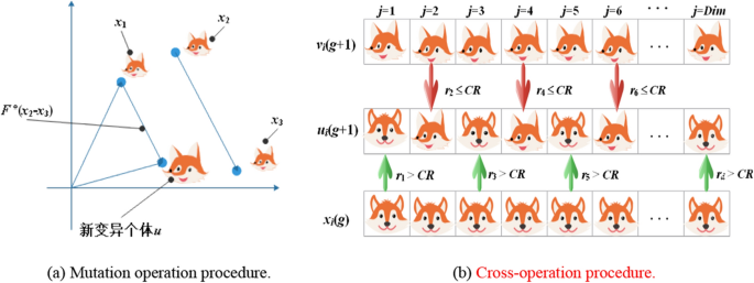
Differential evolution algorithm operation diagram
Some of the previously improved DE are based on Eq. (3.8), and some are based on Eq. (3.9):
$$v_{i} (g + 1) = x_{r1} (g) + F_{1} \cdot (x_{best} (g) - x_{r1} (g)) + F_{2} (x_{r2} (g) - x_{r3} (g)).$$(3.9)In DEMFFA, the formula used for mutation operation is shown in (3.10):
$$v_{i} (g + 1) = x_{r1} (g) + F \cdot ((x_{r2} (g) - x_{r3} (g)) + (x_{r4} (g) - x_{r5} (g))).$$(3.10)In the formula (3.9), \(i \ne r_{1} \ne r_{2} \ne r_{3} \ne r_{4} \ne r_{5}\), the scaling factor is calculated as follows (3.11):
$$F = F_{{\max }} - (iter/Maxiter) \cdot (F_{{\max }} - F_{{\min }} ),$$(3.11)where \(F_{\max }\) is 0.9 and \(F_{\min }\) is 0.4.
-
2)
Cross operation
The g generation population and its variant intermediate individual were cross operated, The formula for the cross operation is shown in (3.12):
$$u_{{i,j}} (g + 1) = \left\{ {\begin{array}{*{20}c} {v_{{i,j}} (g + 1),} & {rand(0,1) \le CR\,or\,j = j_{{rand}} } \\ {x_{{i,j}} (g),} & {otherwise} \\ \end{array} } \right.$$(3.12)where, CR is the crossover probability, and crossover operation uses the crossover probability CR to select \(\{ x_{i} (g)\}\) or \(\{ v_{i} (g + 1)\}\) as the allele of \(\{ u_{i} (g + 1)\}\),\(j_{rand}\) is a random integer \([1,2, \cdots ,D]\), Fig. 6b shows the cross-operation diagram.
In this paper, the CR calculation formula in the formula is shown as (3.13):
$$CR = CR_{\max } - (CR_{\max } - CR_{\min } ) \cdot (iter/Maxiter),$$(3.13)where, \(CR_{\max } = 1\), \(CR_{\min } = 0\), iter is the current iteration number, Maxiter is the total iteration number.
-
3)
Selection operation
Following the execution of the mutation and crossover operations, the DE employs a greedy approach to select the next generation of individuals. This selection process considers both the original individuals and those generated through the crossover operation. The mathematical formula adopted in the selection operation is shown in (3.14):
$$x_{i} (g + 1) = \left\{ {\begin{array}{*{20}l} {u_{i} (g + 1),} & {f(u_{i} (g + 1)) \le f(x_{i} (g))} \\ {x_{i} (g).} & {otherwise} \\ \end{array} } \right.$$(3.14)After adding the differential evolutionary variation strategy to the second stage of FFA, the search range of Fennec foxes is increased, so as to avoid premature stagnation of the algorithm and enhance its ability to jump out of the local optimal.

Steps to improve Fennec Fox algorithm
The original FFA was enhanced by incorporating sin chaotic mapping, cosine adjustment of formula factor, Cauchy operator mutation strategy, and differential evolution mutation strategy. As a result, the improved Fennec Fox algorithm (DEMFFA) was obtained. Compared to the enhanced Fennec Fox algorithm, DEMFFA exhibits stronger searching ability and faster convergence speed. The steps of the DEMFFA, which integrates the aforementioned four strategies are as follows:
-
Step 1. Set the population size pop, the maximum number of iterations T, dimension Dim, and use formula (3.1) to initialize the Fenna fox population. Let the current iteration number \(t = 1\);
-
Step 2. Calculate the fitness value f of Fennec fox, and select the best individual \(X_{best}\), and the optimal fitness value corresponding to the individual is \(f_{best}\);
-
Step 3. In the first stage, the factors of formula (2.5) were adjusted using formula (3.2), and the position of Fennec fox in the first stage was updated using formula (3.3);
-
Step 4. The individual fitness value of Fennec foxes updated in the first stage was calculated, and the best individual \(X_{best}\) and the optimal fitness value \(f_{best}\) corresponding to the individual were updated according to the fitness value;
-
Step 5. Equation (3.7) is used to mutate the individuals generated in the first stage, and the fitness value of the individuals after the mutation is calculated. Compared with the fitness value of Step4, the new most expensive individual \(X_{best}\) and the best fitness value \(f_{best}\) are updated;
-
Step 6. In the second stage, the individual \(x_{rand}\) is randomly generated by Eq. (2.7), the fitness value of the individual is calculated, and the position of the Fennec fox individual in the second stage is generated by Eq. (2.8);
-
Step 7. The fitness value of Fennec fox individuals generated by Step 6 is calculated and compared with the fitness value generated by Step 5. The best individual \(X_{best}\) and the best fitness value \(f_{best}\) are updated;
-
Step 8. Equation (3.10) was used to mutate individuals generated in the first and second stages, and scaling factor F was calculated with Eq. (3.11). The individuals generated by variation are crossed using Eq. (3.12), and the crossover probability CR is calculated using Eq. (3.13). Use formula (3.14) for selection operations.
-
Step 9. The fitness value of Fenna fox individuals generated by variation in Step 8 is calculated and compared with the fitness value generated in Step 7. Finally, the best individual \(X_{best}\) and the best fitness value \(X_{best}\) are updated;
-
Step 10. In case the algorithm reaches the predefined maximum number of iterations, Step 11 is carried out. If the maximum number of iterations is not reached, repeat steps 3 to 9.
-
Step 11. Output the best Fennec fox position \(X_{best}\) and the corresponding fitness value \(f_{best}\) of the best Fennec fox.
According to DEMFFA’s steps, its pseudo-code is shown in Algorithm 2. In addition, Fig. 7 shows the flowchart of DEMFFA.

DEMFFA’s flowchart
DEMFFA algorithm complexity
The algorithm complexity analysis is an approximate estimate, not an exact calculation. It provides a theoretical evaluation of the trend of the increase in the time or space required for the execution of an algorithm, and the algorithm complexity is represented by “O”. The overall algorithm complexity of DEMFFA mainly includes the loop part and the function call part. The function call section includes calls to two functions: the feval function (which calculates the fitness value of the individual at each iteration) and bounds(boundary condition handling). The complexity of the feval function call depends on the complexity of the selected function, and the complexity of this part is \(O(t(f))\).bounds function is a boundary constraint operation on the position of each individual, and its complexity is related to Dim, which is the dimension of the position vector. Generally speaking, the complexity of the function can be regarded as a constant level, which is ignored when calculating the complexity of the algorithm.
Moreover, the computational complexity of the proposed DEMFFA is influenced by various factors, including the initialization process \(Ini\), the maximum number of iterations T, population size N, spatial dimension Dim, and the complexity (O(definition)) of parameter configuration. Sin chaotic mapping is added to the original FFA to process the initial population, and the complexity of the algorithm in this stage is denoted as \(O(Ini)\); In the first stage, the cosine adjustment of the formula factor is added, and the algorithm complexity of this stage is denoted as \(O(\cos { - }adjustment)\); Before the conclusion of the first stage, the Cauchy operator mutation strategy is implemented, and the algorithm complexity of this stage is denoted as \(O(Cauchy{\kern 1pt} {\kern 1pt} operator)\); Finally, differential evolutionary variation strategy is added after the second stage, the complexity of this stage in terms of algorithm is denoted as \(O(DE)\). Thus, the computational complexity of DEMFFA can be described as:

DEMFFA
Numerical experiment and analysis of DEMFFA
In this section, various test functions are utilized to assess the performance of the proposed DEMFFA. Firstly, CEC2017 with higher complexity than the standard function is selected, including 29 functions. Secondly, the newest CEC2022 is selected, which includes 12 single objective test functions. Finally, CEC2020 composed of CEC2014 and CEC2017 is selected, including 10 single objective test functions. Set the population size of all algorithms pop = 30 and the maximum number of iterations T = 1000. In order to eliminate the influence of randomness on each algorithm, set each algorithm to run independently on the test function 20 times.
Comparison of DEMFFA and other optimization algorithms on CEC2017 and CEC2022
In this section, 8 other intelligent optimization algorithms and the original FFA are selected to compare with the proposed DEMFFA. The dimensions of the two test sets are 10, 20. The 8 intelligent optimization algorithms mainly include the following two categories: (1) classical intelligent optimization algorithms: GA [8], PSO [53], DE [9]; (2) Newly proposed optimization algorithms in recent years: GWO [54], GOA [55], BWOA [56], TGA [25], WOA [57]. To differentiate the two optimization algorithms, the Black Widow optimization algorithm is referred to as BWOA. Table 2 shows the parameter settings of some algorithms.
Comparison of DEMFFA and other optimization algorithms on CEC2017
To ensure more reliable and meaningful experimental outcomes, Table 3 presents the comparison results of DEMFFA and other algorithms on CEC2017 benchmark problems, the dimension is set to 10. These metrics encompass the mean, standard deviation (Std), best, worst, and the rank of different algorithms tested on each function (Rank), which is determined by the mean. Table 4 shows the Friedman test results of DEMFFA and the comparison algorithm on CEC2017. Table 5 shows the results of WRST performed by DEMFFA and other algorithms on CEC2017. The best values are represented in bold black. The Wilcoxon rank sum test is denoted as WRST below.
The performance comparison presented in Table 3 indicates that DEMFFA exhibits superior performance when compared to other similar algorithms. On the whole, DEMFFA won first place in 20 of the 29 test functions, showing obvious superiority. In solving unimodal and simple multi-modal functions, DEMFFA is superior to other algorithms on F1, F4, F6, and F9. Although the performance of DEMFFA on F7 and F10 is not as good as that of GWO, which ranks second, its standard deviation is the smallest, which proves that DEMFFA's performance is stable. There are obvious advantages for mixed and combined functions. This indicates that the inclusion of sin chaotic mapping, cosine adjustment of formula factors, Cauchy operator mutation strategy, and differential evolution mutation strategy effectively enhances the algorithm's search capability. Furthermore, it substantiates that the proposed DEMFFA possesses strong exploration ability and is capable of avoiding local optima.
When proposing a new algorithm, we need to know how the proposed algorithm compares to the existing algorithm, and we need to use the method of model performance evaluation. Among them, the Friedman test is a method, which is characterized by multiple algorithm comparisons. When the performance of the compared algorithms is similar, their average sequence values will be the same. Table 4 clearly illustrates that the proposed DEMFFA demonstrates optimal performance on the majority of test functions, especially on hybrid function and composition functions. On F6 and F16, DEMFFA has the same performance as GWO, which ranks second overall, and their Friedman test values are the same. To determine the final Friedman test ranking results, the values obtained from the Friedman test results of 20 independent runs were sorted. DEMFFA emerged in first place across 21 test functions. In comparison to others, DEMFFA achieved an average ranking of 1.2759, securing the top position overall. This conclusive evidence confirms that the proposed algorithm demonstrates superior average performance.
In addition to the above methods to test the performance of algorithms, there are WRST. Table 5 shows the results of the WRST between DEMFFA and other comparison algorithms in the CEC2017 test set. The last line “+/ = /−” shows the test results. ‘+’ indicates that the performance of the compared algorithm is better than DEMFFA on this test function; ‘−’ indicates that the performance of the compared algorithm is worse than that of DEMFFA on this test function; ‘=’ indicates that the performance of the compared algorithm on this test function is similar to that of the proposed DEMFFA. According to the data in the last row of Table 5, the WRST test result of GWO is 4/2/23, indicating that DEMFFA performs worse than GWO in four functions, namely F5, F10, F16, and F23. There is not much difference in performance between the two functions; The proposed DEMFFA performs better than GWO on most of the 23 functions. The WRST test results of DE, GA, GOA, WOA, and FFA are all 0/0/29. It can be concluded that DEMFFA is very competitive in the comparison of these functions in the CEC2017 test set, which also indicates that DEMFFA is superior to FFA in 29 functions. It shows that the improved algorithm improves the performance of the original algorithm. The test results of BWOA and TGA are 0/1/28, indicating that DEMFFA and they show the same performance on one function and better performance on the other functions.
As can be seen from the convergence curve in Fig. 8, DEMFFA’s convergence curve tends to be stable and basically tends to a fixed value as the number of iterations increases. It is not difficult to find that most of the convergence curves of the proposed DEMFFA are kept below the convergence curves of other algorithms, and the convergence speed is faster and the solving ability is better than that of other comparison algorithms. Especially in F13, F18, F19, F21, F22, F24, F30 the effect is more obvious. For FFA, functions F3, F7, F9, and F14 converge prematurely, and their corresponding convergence curves tend to flatten out when the number of iterations is about 200, indicating that FFA at this time may fall into local optimality. The improved FFA greatly improves the performance, convergence speed, and convergence accuracy of the algorithm, and effectively prevents the algorithm from falling into the local optimal prematurely. The primary advantage of the boxplot is its resilience to outliers, allowing it to provide a stable representation of the discrete distribution of data. From the comparison of algorithms in Fig. 9 with the boxplot, the proposed DEMFFA has lower and narrower boxes and a smaller median for most functions.


Convergence curve of DEMFFA and other comparison algorithms in CEC2017


Box plot of DEMFFA and other comparison algorithms in CEC2017
In general, DEMFFA has fewer outliers than other algorithms. The performance order of DEMFFA and other algorithms compared is as follows: DEMFFA > GWO > PSO > TGA > WOA > FFA > DE > GOA > BWOA > GA. Overall, the proposed DEMFFA demonstrates superior performance compared to other comparison algorithms when assessed on CEC2017.
Comparison of DEMFFA and other optimization algorithms on CEC2022
Apart from the evaluation on CEC2017, the DEMFFA and other comparison algorithms were also examined on CEC2022, the dimension is set to 20. Table 6 shows the comparison results between DEMFFA and other algorithms in CEC2022. Table 7 displays the Friedman test outcomes for DEMFFA and the comparison algorithm on the CEC2022. Meanwhile, Table 8 illustrates the results of the WRST conducted by DEMFFA and the other algorithms on the same test set. The text presented in black font holds the same interpretation as previously discussed.
The findings presented in Table 6 demonstrate that DEMFFA outperforms alternative algorithms in terms of performance. On the whole, DEMFFA has achieved first place in half of the 12 test functions, showing obvious superiority. Table 6 clearly illustrates that the proposed DEMFFA exhibits exceptional performance across all 6 test functions, especially on mixed functions and combined functions. On the F7-F10, DEMFFA’s effect is even more pronounced. In Table 7, the values of Friedman test results of 20 independent runs are used to rank and obtain the final ranking results. Compared with other algorithms, DEMFFA’s average ranking is 1.8333, ranking first overall, which proves that the proposed algorithm has the best average performance.
The value of WRST of DEMFFA and other comparison algorithms on the CEC2022 test set is given in Table 8. The last line “+/ = /−” gives the statistical result of the test, and the meaning of the specific symbol is the same as that in the previous section. According to the data in the last row of Table 8, WRST results of DE, GA, GOA, TGA, WOA, and BWOA are all 0/0/12, indicating that compared with these algorithms, the proposed DEMFFFA is superior to these algorithms in 12 test functions on the CEC2022 test set. The WRST results of PSO are 1/0/11, indicating that PSO is superior to DEMFFA in one of the 12 functions. The WRST test result of GWO is 1/1/10, indicating that, compared with GWO, DEMFFA’s performance in one function is worse than that of the proposed algorithm, and its performance in one function is similar to that of the proposed algorithm, they are F4 and F6 respectively. Compared with the original algorithm FFA, the result of the rank sum test is 0/1/11, and the proposed DEMFFA is superior to the original algorithm in 11 test functions, which indicates that the improved algorithm improves the performance of the original algorithm.
As can be seen from the convergence curve in Fig. 10, as the number of iterations increases, the convergence curve of DEMFFA proposed is mostly kept below the convergence curve of other algorithms, with faster convergence speed and better solving ability than other comparison algorithms. Especially on F7, F9, and F12, the effect is more obvious. In addition, on F1, F7, and F9, the original FFA converges prematurely, resulting in the algorithm failing to find the optimal solution, while the improved FFA algorithm greatly improves the performance, convergence speed, and convergence accuracy of the algorithm, effectively avoiding the algorithm falling into the local optimal prematurely. From Fig. 11 with the boxplot, the observed characteristics indicate that the proposed DEMFFA algorithm generally exhibits lower and narrower boxes, as well as smaller median values, for the majority of functions. In general, DEMFFA has fewer outliers than other algorithms. In the CEC2022, the performance order of DEMFFA and other algorithms compared is as follows: DEMFFA > GWO > PSO > WOA > TGA > FFA > DE > GOA > BWOA > GA. Overall, the proposed DEMFFA outperforms other comparison algorithms on the CEC2022.

Convergence curve of DEMFFA and other comparison algorithms in CEC2022

Box plot of DEMFFA and other comparison algorithms in CEC2022
Comparison of DEMFFA and other optimization algorithms on the CEC2020
In the previous section, DEMFFA and the selected comparison algorithm were quantitatively analyzed on CEC2022 and CEC2017 test sets. In this section, we first conducted a qualitative analysis of DEMFFA on CEC2020 test sets. Four indicators are selected for qualitative analysis. The results of qualitative analysis are shown in Fig. 12. Secondly, DEMFFA was quantitatively analyzed with the 12 algorithms selected as follows: (1) Improved classical intelligent optimization algorithms: improved Particle swarm optimization algorithm (HCLPSO) [58], improved Golden Jackal optimization algorithm (IGJO) [59], improved Gray Wolf optimization algorithm (IGWO) [60]; (2) Newly proposed optimization algorithms in recent years: Archimedes Optimization algorithm (AOA) [61], Crayfish Optimization Algorithm (COA) [24], Kepler Optimization Algorithm (KOA) [16], Seahorse Optimization algorithm (SHO) [6], Spider bee Optimization algorithm (SWO) [62], Genghis Khan Shark Optimization Algorithm (GKSO) [33], Human Memory Optimization algorithm (HMO) [63], Triangulation Topology Aggregation Optimizer (TTAO) [64], and the parameters of the comparison algorithm are shown in Table 9.

DEMFFA’s qualitative analysis results on the CEC2020 test set
In Fig. 12, the first column is the image of the corresponding function on the CEC2020 test set, and the second column is the position of the Fennec fox individual during the search iteration process. It can be seen from the second column that Fennec foxes are evenly distributed in the search space, and with the increase of iteration times, Fennec foxes will converge to the optimal individuals, and this feature is most obvious on F2, F4, F8, and F10. Different individuals will converge toward the optimal solution, which indicates that DEMFFA’s optimization ability and convergence have shown great advantages. At the same time, the search ability of the algorithm is also different for different search Spaces.
It can be seen from the third column of the Fennec fox individual search track that the Fennec fox individual fluctuates greatly in the early stage of search iteration, indicating that the Fennec fox individual has strong exploration ability. In the later iteration period, the individual fluctuation amplitude of Fennec foxes was small and tended to be flat, reflecting good development ability. It can be seen from the convergence curve in the fourth column that DEMFFA, after continuous iteration in the early stage, the fitness function value keeps decreasing, and finally reaches the convergence state and finds the optimal solution. On the functions F8 and F10, the convergence curves converge faster, showing good performance. In addition, the average fitness value curve of the fifth column shows a decreasing trend and finally reaches a convergence state. From the results of qualitative analysis, DEMFFA greatly improves the performance of the original algorithm.
Tables 10, 11, 12 shows the results of DEMFFA and 12 comparison algorithms independently running 20 times on the 20 dimensions of the CEC2020 test set. The meanings represented by the letters in the table are the same as in the previous section, and the optimal value of DEMFFA is marked in black in bold. As can be seen from Table 10, among the 10 test functions of CEC2020, the DEMFFA achieved first place in 7 functions, proving that DEMFFA’s performance is better than other comparison algorithms, and the first functions are F2-F7 and F10. The performance of DEMFFA is not as good as GKSO, HMO, TTAO, and COA in solving the function F1, but it is stronger than other comparison algorithms. DEMFFA ranks first with an average rank of 1.6, followed by GKSO with a rank of 2.5. In the CEC2020 test set, the performance ranking of the algorithms is as follows: DEMFFA > GKSO > TTAO = PSO > IGJO > HMO > SHO > IGWO > AOA > S.
WO > KOA > FFA, it can be seen that the added strategy greatly improves the performance of the original algorithm.
Table 11 shows the Friedman test results of DEMFFA and the comparison algorithm on the CEC2020 test set, and the optimal Friedman test values are marked in black in bold. As can be seen from Table 10, the proposed DEMFFA has the smallest Friedman test value on most test functions, showing the optimal performance, especially on basic functions and mixed functions. On function F4, DEMFFA has the same Friedman test value as GKSO, FFA, SHO, AOA, COA, and IGJO, showing the same performance. Table 12 shows the WRST results of DEMFFA and other algorithms, and the meanings represented by symbols in the table are the same as in the previous section. It can be seen that the WRST results of HCLPSO, IGWO, KOA, SWO, and TTAO are 0/0/10, indicating that the proposed algorithm on the 10 functions on the CEC2020 test set is better than the compared algorithm. The WRST results of IGJO, COA, and GKSO are 0/2/8, indicating that DEMFFA has shown the same performance as these algorithms in the two functions compared with these algorithms. In addition, the results of AOA, SHO, FFA, and HMOde WRST are 0/1/9, indicating that DEMFFA shows the same performance as the comparison algorithm in one function when comparing these algorithms. No algorithm performs better than the proposed algorithm on the CEC2020 test set.
Figures 13, 14, 15 shows the convergence diagram, box plot, and radar diagram of DEMFFA and the comparison algorithm CEC2020 test set. As can be seen from the convergence curve in Fig. 13, the convergence curve of the proposed DEMFFA is mostly kept at the lower left of the convergence curve of other algorithms, with faster convergence speed and better solving ability than other comparison algorithms. Compared with the original FFA algorithm, the optimization ability of the proposed DEMFFA is greatly improved, especially on F2, F5, F8, and F10. Because FFA falls into local optimal too early, it cannot find the optimal solution, and the promoted DEMFFA avoids this problem. As can be seen from the box diagram in Fig. 14, the box corresponding to DEMFFA is shorter and has fewer abnormal points, indicating that the proposed DEMFFA is relatively stable and its performance has been greatly improved. The radar in Fig. 15 shows the comparison between DEMFFA and each algorithm. It can be seen that, compared with other algorithms, DEMFFA has the smallest shadow area corresponding to the radar map, which also shows that several strategies added have a great effect on improving the performance of FFA.

Convergence curve of DEMFFA and other algorithms on CEC2020

Box plot of DEMFFA and other algorithms on CEC2020

Radar diagram of DEMFFA and other algorithms on CEC2020
DEMFFA is applied to engineering optimization problems
In addition to evaluating the algorithm's performance using various test sets, it is also valuable to assess its effectiveness by applying it to real-world engineering design problems. By doing so, we can gauge the algorithm's ability to tackle complex, practical optimization challenges. This approach provides a more comprehensive evaluation and validates the algorithm's applicability in real-life scenarios. In this section, ten engineering design problems are selected to test the DEMFFA, including mechanical design problems, process design problems, and synthesis problems. Specific engineering design problems are tension/compression spring design problems, process synthesis problems, Hydrodynamic thrust bearing design problems, Himmelblau function problems, etc. The variable for each question is denoted with the first letter Ff of the Fennec fox English word. The algorithms compared in this section are: DE [9], PSO [53], AOA [61], COA [24], SHO[6], IGWO [60], BWOA [56], FFA [48].
Welding beam design problems
This problem focuses on minimizing the manufacturing cost while adhering to specific constraints. The primary objective is to optimize the design parameters of the welding beam to achieve the most cost-efficient solution. This study recorded the thickness, height, and length of the welded beam, as well as the thickness of the weld, denoted as variables \(Ff_{1}\)、\(Ff_{2}\)、\(Ff_{3}\)、\(Ff_{4}\), respectively. Figure 16 illustrates the structural diagram of this problem. The mathematical model of the problem considering variables \(x = [Ff_{1} ,Ff_{2} ,Ff_{3} ,Ff_{4} ]\) is as follows:

Schematic diagram planning for welding beam design issue
Make:
\(g_{1} (Ff) = H(Ff) - H_{\max } \le 0\), \(g_{2} (Ff) = \sigma (Ff) - M_{\max } \le 0\), \(g_{3} (Ff) = \delta (Ff) - \delta_{\max } \le 0\).
\(g_{4} (Ff) = Ff_{1} - Ff_{4} \le 0\), \(g_{5} (Ff) = 0.125 - Ff_{1} \le 0\), \(g_{6} (Ff) = Q - Q_{c} (Ff) \le 0\).
\(g_{7} (Ff) = 1.10471Ff_{1}^{2} + 0.04811Ff_{3} Ff_{4} (14 + Ff_{2} ) - 5 \le 0\),
In formula, \(Q = 6000\;lb\), \(L = 14\;{\text{in}}\), \(D = 30 \times 10^{6} \;{\text{psi}}\), \(S = 12 \times 10^{6} {\kern 1pt} {\kern 1pt} {\text{psi}}\), \(M_{\max } = 30000\,{\text{psi}}\),
\(H_{\max } = 136000{\kern 1pt} {\kern 1pt} {\kern 1pt} {\kern 1pt} {\text{psi}}\), \(\delta_{\max } = 0.25{\kern 1pt} {\kern 1pt} {\kern 1pt} {\text{in}}\), \({0}{\text{.1}} \le Ff_{1} \le 2\), \(0.1 \le Ff_{2} \le 10\), \(0.1 \le Ff_{3} \le 10\), \(\;{0}{\text{.1}} \le Ff_{4} \le 2\).
Other parameters are as follows:
\(H(x) = \sqrt {(H^{\prime} )^{2} + 2H{\prime} H^{^{\prime\prime}} \frac{{x_{2} }}{2R} + (H^{^{\prime\prime}} )^{2} }\), \(H^{\prime} = \frac{Q}{{\sqrt 2 Ff_{1} Ff_{2} }}\), \(H^{^{\prime\prime}} = \frac{MR}{J}\), \(M = Q(L + \frac{{Ff_{2} }}{2})\),
\(R = \sqrt {\frac{{Ff_{2}^{2} }}{4} + (\frac{{Ff_{1} + Ff_{3} }}{2})^{2} }\), \(J = 2((\frac{{Ff_{2}^{2} }}{12} + (\frac{{Ff_{1} + Ff_{3} }}{2})^{2} ) \cdot \sqrt 2 Ff_{1} Ff_{2} )\), \(M(Ff) = \frac{6QL}{{Ff_{4} Ff_{3}^{2} }}\), \(\delta (Ff) = \frac{4QL}{{DFf_{4} Ff_{3}^{3} }}\), \(Q_{c} = (1 - \frac{{Ff^{3} }}{2L}\sqrt{\frac{D}{4S}} )\frac{{4.013\sqrt {DSFf_{3}^{2} Ff_{4}^{6} /36} }}{{L^{2} }}\).
DEMFFA and several other intelligent optimization algorithms were used for this problem. The number of iterations to solve the problem was 500, the number of the population was 30, and the results were obtained by independent operation 20 times. The solution outcomes are presented in Table 13, while the operational statistical findings are depicted in Table 14. The optimum values are denoted by the bolded entries within the table. The comparative analysis in Table 13 demonstrates the significant advantages of DEMFFA in addressing welded beam engineering challenges, with the minimum cost recorded as 1.767016102. Furthermore, the observations from Table 14 reveal that DEMFFA exhibits superior stability, as reflected by its minimal standard deviation.
Three-bar truss design problem
Three-bar truss is a common structural form, that is widely used in Bridges, buildings, and mechanical equipment. The design optimization of the three-bar truss means that the structure has the best performance and economy under certain constraints by adjusting the parameters of the size, shape, and connection mode of the bar. The structural diagram of the three-bar truss problem is shown in Fig. 17. Considering variables \(x = [Ff_{1} ,Ff_{2} ] = [x_{1} ,x_{2} ]\), the specific mathematical model is as follows:

Schematic diagram of three-bar truss design problem
Make:
\(g_{1} (Ff) = \frac{{\sqrt 2 Ff_{1} + Ff_{2} }}{{\sqrt 2 Ff_{1}^{2} + 2Ff_{1} Ff_{2} }}Q - H \le 0\), \(g_{2} (Ff) = \frac{{Ff_{2} }}{{\sqrt 2 Ff_{1}^{2} + 2Ff_{1} Ff_{2} }}Q - H \le 0\),
\(g_{3} (Ff) = \frac{1}{{\sqrt 2 Ff_{2} + Ff_{1} }}Q - H \le 0\).
In the formula, the value range of the variable is:
\(0 \le Ff_{1} \le 1\), \(0 \le Ff_{2} \le 1\).
Other parameters are:
\(l = 100{\text{cm}}\), \(Q = 2{\text{kN}}/{\text{cm}}^{2}\), \(H = 2{\text{kN}}/{\text{cm}}^{2}\).
The optimization problem was tackled using the DEMFFA along with several other intelligent optimization algorithms. The respective results obtained are illustrated in Table 15. Furthermore, Table 16 presents the statistical outcomes derived from 20 independent runs conducted using different algorithms. Bold data is the optimal value. It can be seen from Table 15 that DEMFFA obtains the minimum value in solving the design problem of the three-bar truss, and the cost is less than that of the compared algorithm, and the cost is the smallest, the minimum cost is 263.463431. Furthermore, an examination of Table 16 demonstrates that DEMFFA exhibits the lowest standard deviation among the algorithms, which implies that it showcases strong stability in resolving this particular problem.
Tension/compression spring design
This problem primarily involves optimizing three continuous decision variables while satisfying four constraints. Figure 18 displays the schematic diagram. In this problem, the mathematical model, taking into account the variables \(x = [Ff_{1} ,Ff_{2} ,Ff_{3} ] = [d,D,P]\), is precisely defined as follows:

Tension/compression spring design
Make:
\(g_{1} (Ff) = 1 - \frac{{Ff_{2}^{3} Ff_{3} }}{{71785Ff_{1}^{4} }} \le 0\), \(g_{2} (Ff) = \frac{1}{{5108Ff_{1}^{2} }} + \frac{{4Ff_{2}^{2} - Ff_{1} Ff_{2} }}{{12566(Ff_{2} Ff_{1}^{3} - Ff_{1}^{4} )}} - 1 \le 0\),
\(g_{3} (Ff) = 1 - \frac{{140.45Ff_{1} }}{{Ff_{2}^{2} Ff_{3} }} \le 0\), \(g_{4} (Ff) = \frac{{Ff_{1} + Ff_{2} }}{1.5} - 1 \le 0\),
In the formula, the value range of the variable is:
\(0.05 \le Ff_{1} \le 2\), \(0.25 \le Ff_{2} \le 1.3\), \(2 \le Ff_{3} \le 15\).
To address the optimization problem aiming for minimization, the DEMFFA and other intelligent optimization algorithms for solution exploration. The outcomes of the DEMFFA algorithm and other comparative algorithms in resolving this problem are presented in Table 17. Table 18 displays the statistical analysis of the DEMFFA and several other algorithms after conducting 20 independent runs, with the optimum value being depicted in bold. The examination of Table 17 reveals that the DEMFFA algorithm achieves the lowest value in resolving this problem, with the minimum cost recorded as 0.012668647. Furthermore, from Table 18, it is clear that DEMFFA demonstrates the lowest standard deviation when compared to the other algorithms. This emphasizes the algorithm’s noteworthy performance in efficiently addressing this problem.
Hydrodynamic thrust bearing design
The goal of the hydrodynamic thrust bearing design problem [65] is to minimize power loss. In addition, this problem involves several constraints which include considerations such as bearing capacity and other physical limitations. Figure 19 illustrates the structural diagram of the hydrodynamic thrust bearing design, variable in consideration \(x = [Ff_{1} ,Ff_{2} ,Ff_{3} ,Ff_{4} ]\). The specific mathematical model is as follows:

Schematic diagram of the design structure of hydrodynamic thrust bearing
Make:
\(g_{1} (Ff) = W - W_{s} \ge 0\), \(g_{2} (Ff) = H_{\max } - H_{0} \ge 0\),
\(g_{3} (Ff) = \Delta T_{\max } - \Delta T \ge 0\), \(g_{4} (Ff) = h - h_{\min } \ge 0\),
\(g_{5} (Ff) = Ff_{1} - Ff_{2} \ge 0\), \(g_{6} (Ff) = 0.001 - \frac{\alpha }{{gH_{0} }}(\frac{{Ff_{4} }}{{2\pi Ff_{1} h}}) \ge 0\),
\(g_{7} (Ff) = 5000 - \frac{W}{{\pi (Ff_{1}^{2} - Ff_{2}^{2} )}} \ge 0\),
where, \(W = \frac{{\pi H_{0} }}{2}\frac{{Ff_{1}^{2} - Ff_{2}^{2} }}{{\ln \frac{{Ff_{1} }}{{Ff_{2} }}}}\), \(H_{0} = \frac{{6Ff_{3} Ff_{4} }}{{\pi h^{3} }}\ln \frac{{Ff_{1} }}{{Ff_{2} }}\), \(E_{f} = 9336Ff_{4} \alpha D\Delta T\), \(\Delta T = 2(10^{H} - 560)\), \(H = \frac{{\log_{10} \log_{10} (8.122e6Ff_{3} + 0.8) - D_{1} }}{n}\), \(h = (\frac{2\pi M}{{60}})^{2} \frac{{2\pi Ff_{3} }}{{E_{f} }}(\frac{{Ff_{1}^{4} }}{4} - \frac{{Ff_{2}^{4} }}{4})\).
Variable values range from:
\(1 \le Ff_{1} ,Ff_{2} ,Ff_{4} \le 16\), \(1e - 6 \le Ff_{3} \le 16e - 6\).
Other parameters in the formula are: \(\alpha = 0.0307\), \(D = 0.5\), \(n = - 3.55\), \(D_{1} = 10.04\), \(W_{s} = 101000\), \(H_{\max } = 1000\), \(\Delta T_{\max } = 50\), \(h_{\min } = 0.001\), \(g = 386.4\), \(M = 750\).
To solve this problem of minimizing loss, the DEMFFA and various other intelligent algorithms are utilized. Table 19 shows the results of DEMFFA and others to solve this problem. The statistical results of DEMFFA and different algorithms are presented in Table 20. It can be seen from Table 19 that the DEMFFA achieves the minimum loss in solving the design problem of hydraulic thrust bearing, and the minimum loss is 7696.981009. Furthermore, an examination of Table 20 reveals that DEMFFA exhibits the smallest standard deviation among the algorithms, suggesting that it is highly competitive in the design of hydraulic thrust bearings.
Cantilever beam design
The cantilever beam design problem consists of five square hollow elements and is a nonlinear constrained optimization problem. As depicted in Fig. 20, each element is characterized by a variable, while its thickness remains constant. The side length of the first cross-section square is \(x_{1}\), and so on, so the problem involves a total of five variables, that is, there are five decision variables, and a constraint condition of vertical displacement needs to be satisfied. Considering variables \(x = [Ff_{1} ,Ff_{2} ,Ff_{3} ,Ff_{4} ,Ff_{5} ]\), the mathematical model for this problem is as follows:

Structure diagram of cantilever beam
The constraint condition is:
\(g(Ff) = \frac{61}{{Ff_{1}^{3} }} + \frac{37}{{Ff_{2}^{3} }} + \frac{19}{{Ff_{3}^{3} }} + \frac{7}{{Ff_{4}^{3} }} + \frac{1}{{Ff_{5}^{3} }} \le 0\),
The value range of the variable is:
\(0.01 \le Ff_{1} ,Ff_{2} ,Ff_{3} ,Ff_{4} ,Ff_{5} \le 100\),
This problem is addressed by employing the selected comparison algorithms, the outcomes of these algorithms are compared with those of the enhanced DEMFFA. Table 21 displays the comparison results of all algorithms, and Table 22 presents the statistical outcomes of all algorithms after 20 independent runs. The optimal data is highlighted in bold. Table 21 showcases the optimal values achieved by different algorithms for solving this problem, along with the corresponding decision variable values. DEMFFA has attained the minimum value in this problem, with a minimum weight of 1.336069686. Upon examining the statistical results presented in Table 22, it is evident that DEMFFA’s solution to the cantilever beam problem exhibits the smallest standard deviation, best value, worst value, and average value. This indicates that DEMFFA’s algorithm demonstrates a stable performance in solving this particular problem.
Gas transmission compressor design
The purpose of the gas transmission compressor design problem is to minimize the total cost of transporting natural gas. The constraint condition that each variable is greater than 0 is required. The structural diagram of the gas transmission compressor is shown in Fig. 21. Set the variable involved in this question to \(x = [Ff_{1} ,Ff_{2} ,Ff_{3} ] = [L,P,R]\), the mathematical model for this problem can be expressed as follows:

Structure diagram of gas transmission compressor
The constraint condition is:
\(Ff_{1} ,Ff_{2} ,Ff_{3} > 0\),
Variable values range from:
\(10 \le Ff_{1} \le 55\), \(1.1 \le Ff_{2} \le 2\), \(10 \le Ff_{3} \le 40\).
The selected comparison algorithms are utilized to address this problem, and the results obtained from these algorithms are compared with improved DEMFFA. Table 23 displays the comparison results of all algorithms, including the optimal values obtained to solve this problem, along with the corresponding decision variable values. Table 24 presents the statistical results of all algorithms after 20 independent runs, with the optimal data highlighted in bold. From the outcomes presented in Table 23, it is clear that DEMFFA has achieved the lowest value in the gas transmission compressor problem, with a minimum transportation cost of 2,964,375.509. Furthermore, the statistical outcomes presented in Table 24 reveal that DEMFFA’s solution to the design problem of this problem exhibits the smallest standard deviation, best value, worst value, and average value. This indicates that DEMFFA demonstrates relatively accurate performance and good stability in resolving this problem.
Process synthesis problem
The chemical process synthesis problem belongs to the process design and synthesis problem [66]. This problem mainly includes one constraint condition and two decision variables \(x_{1}\), \(x_{2}\). Variables are considered in this problem \(x = [Ff_{1} ,Ff_{2} ] = [x_{1} ,x_{2} ]\), and the specific mathematical model for the process synthesis problem can be presented below:
Make:
\(g_{1} (Ff) = - Ff_{1}^{2} - Ff_{2} + 1.25 \le 0\), \(g_{2} (x) = Ff_{1} + Ff_{2} \le 1.6\),
Variable values range from:
\(0 \le Ff_{1} \le 1.6\), \(0 \le Ff_{2} \le 1\).
The process synthesis problem was addressed by employing the DEMFFA along with selected comparison algorithms. Subsequently, a comprehensive comparison was conducted to evaluate and analyze the results produced by these algorithms. Table 25 displays the comparison results of all algorithms employed to solve the process synthesis problem, along with their corresponding decision variable values. The optimal value obtained by each algorithm is highlighted in bold. Additionally, Table 26 presents the statistical results of all algorithms after conducting 20 independent runs. From the analysis of Table 25, it is evident that the DEMFFA achieved the minimum value of 1.998997992 for the process synthesis problem. The corresponding results in Table 26 presenting the statistical outcomes further demonstrate that DEMFFA exhibits the smallest standard deviation, best value, worst value, and average value among all algorithms used to solve the comprehensive chemical process problem, indicating its superior competence in addressing this specific problem.
Himmelblau’s function problem
Himmelblau is used as a universal benchmark for analyzing nonlinear constraint optimization algorithms [66]. The problem contains 6 nonlinear constraints and five variables. Considering the variables \(x = [Ff_{1} ,Ff_{2} ,Ff_{3} ,Ff_{4} ,Ff_{5} ]\), the specific mathematical model for the Himmelblau function problem can be represented as follows:
The constraint condition is:
\(g_{1} (Ff) = - G_{1} \le 0\), \(g_{2} (Ff) = G_{1} - 92 \le 0\), \(g_{3} (Ff) = 90 - G_{2} \le 0\),
\(g_{4} (Ff) = G_{2} - 110 \le 0\), \(g_{5} (Ff) = 20 - G_{3} \le 0\), \(g_{6} (Ff) = G_{3} - 25 \le 0\),
Other parameters in the formula are:
\(G_{1} = 85.334407 + 0.0056858Ff_{2} Ff_{5} + 0.0006262Ff_{1} Ff_{4} - 0.0022053Ff_{3} Ff_{5}\),
\(G_{2} = 80.51249 + 0.0071317Ff_{2} Ff_{5} + 0.0029955Ff_{1} Ff_{2} + 0.0021813Ff_{3}^{2}\),
\(G_{3} = 9.300961 + 0.0047026Ff_{3} Ff_{5} + 0.00125447Ff_{1} Ff_{3} + 0.0019085Ff_{3} Ff_{4}\),
Variable values range from:
\(78 \le Ff_{1} \le 102\), \(33 \le Ff_{2} \le 45\), \(27 \le Ff_{3} \le 45\),
\(27 \le Ff_{4} \le 45\), \(27 \le Ff_{5} \le 45\).
The Himmelblau's function problem was addressed using the DEMFFA along with selected comparison algorithms. The results of these algorithms were then compared. Table 27 presents the comparison results of all algorithms, showcasing the optimal value obtained by different algorithms in solving this problem, along with their corresponding variable values. Bold data represents the optimal value. Additionally, Table 28 displays the statistical results of all algorithms. It can be seen that DEMFFA obtained the minimum value on this problem, and the minimum value was 140,996.5484. In Table 28, the standard deviation, the best value, worst value and average value of DEMFFA in solving the comprehensive problem of the chemical process are all the smallest, indicating that DEMFFA has great advantages.
Reducer design problems
Reducer design is an engineering design problem. To make the weight of the reducer as small as possible. Figure 22 is the structural diagram of the reducer. Consider the variables involved in this problem:\(x = [Ff_{1} ,Ff_{2} ,Ff_{3} ,Ff_{4} ,Ff_{5} ,Ff_{6} ,Ff_{7} ]\), the mathematical model is as follows:

Structure diagram of the reducer
The constraint condition is:
\(g_{1} (Ff) = \frac{27}{{Ff_{1} Ff_{2}^{2} Ff_{3} }} - 1 \le 0\), \(g_{2} (Ff) = \frac{397.5}{{Ff_{1} Ff_{2}^{2} Ff_{3}^{2} }} - 1 \le 0\), \(g_{3} (Ff) = \frac{{1.93Ff_{4}^{3} }}{{Ff_{2} Ff_{6}^{4} Ff_{3} }} - 1 \le 0\),
\(g_{4} (Ff) = \frac{{1.93Ff_{5}^{3} }}{{Ff_{2} Ff_{7}^{4} Ff_{3} }} - 1 \le 0\), \(g_{5} (Ff) = \frac{{[(745({{Ff_{4} } \mathord{\left/ {\vphantom {{Ff_{4} } {Ff_{2} Ff_{3} }}} \right. \kern-0pt} {Ff_{2} Ff_{3} }}))^{2} + 16.9 \times 10^{6} ]^{0.5} }}{{110Ff_{6}^{3} }} - 1 \le 0\),
\(g_{6} (Ff) = \frac{{[(745({{Ff_{5} } \mathord{\left/ {\vphantom {{Ff_{5} } {Ff_{2} Ff_{3} }}} \right. \kern-0pt} {Ff_{2} Ff_{3} }}))^{2} + 157.5 \times 10^{6} ]^{0.5} }}{{85Ff_{7}^{3} }} - 1 \le 0\), \(g_{7} (Ff) = \frac{{Ff_{2} Ff_{3} }}{40} - 1 \le 0\),
\(g_{8} (Ff) = \frac{{5Ff_{2} }}{{Ff_{1} }} - 1 \le 0\), \(g_{9} (Ff) = \frac{{Ff_{1} }}{{12Ff_{2} }} - 1 \le 0\), \(g_{10} (Ff) = \frac{{1.5Ff_{6} + 1.9}}{{Ff_{4} }} - 1 \le 0\),
\(g_{11} (Ff) = \frac{{1.1Ff_{7} + 1.9}}{{Ff_{5} }} - 1 \le 0\),
Variable values range from:
\(2.6 \le Ff_{1} \le 3.6\), \(0.7 \le Ff_{2} \le 0.8\), \(17 \le Ff_{3} \le 28\), \(7.3 \le Ff_{4} ,Ff_{5} \le 8.3\),
\(2.9 \le Ff_{6} \le 3.9\), \(5.0 \le Ff_{7} \le 5.5\).
The reducer design problem was approached using the DEMFFA in conjunction with a chosen comparison algorithm. A comparison of the results obtained by these algorithms is presented in Table 29. This table showcases the outcome of different algorithms in solving the reducer design problem, highlighting the optimal value achieved. The corresponding statistical results of all algorithms, after conducting 20 independent runs, are displayed in Table 30. In both tables, the optimal value is indicated in bold. Table 29 displays the optimal value achieved by different algorithms in solving this problem, along with the corresponding variable value. It is noteworthy that the DEMFFA obtained the lowest value, which is 2996.3508. As for the statistical results indicated in Table 30, while the standard deviation of DEMFFA is not the smallest, it boasts the best, worst, and average values among all algorithms in solving this problem. This suggests that the DEMFFA remains highly competitive and efficient in addressing this particular problem.
Stepped cantilever beam design
A stepped cantilever is similar to a cantilever design problem in that the aim is to keep its total weight as small as possible while meeting the maximum load. This problem needs to meet eleven constraints, involving ten variables, and optimize the corresponding parameters to get the minimum weight of the stepped cantilever beam, which is more complicated than the cantilever beam design. Figure 23 shows the structural diagram of the stepped cantilever beam. Consider the variables in this problem:\(x = [Ff_{1} ,Ff_{2} ,Ff_{3} ,Ff_{4} ,Ff_{5} ,Ff_{6} ,Ff_{7} ,Ff_{8} ,Ff_{9} ,Ff_{10} ]\), the specific mathematical model of this problem is as follows:

Structure diagram of the stepped cantilever beam
The constraint condition is:
\(g_{1} (Ff) = \frac{6Pl}{{Ff_{9} Ff_{10}^{2} }} - \sigma_{\max } \le 0\), \(g_{2} (Ff) = \frac{6Pl}{{Ff_{7} Ff_{8}^{2} }} - \sigma_{\max } \le 0\), \(g_{3} (Ff) = \frac{6Pl}{{Ff_{5} Ff_{6}^{2} }} - \sigma_{\max } \le 0\),
\(g_{4} (Ff) = \frac{6Pl}{{Ff_{3} Ff_{4}^{2} }} - \sigma_{\max } \le 0\), \(g_{5} (Ff) = \frac{6Pl}{{Ff_{1} Ff_{2}^{2} }} - \sigma_{\max } \le 0\),
\(g_{6} (Ff) = \frac{{Pl^{3} }}{{Ff_{3} Ff_{4}^{2} }}(\frac{244}{{Ff_{1} Ff_{2}^{3} }} + \frac{148}{{Ff_{3} Ff_{4}^{3} }} + \frac{76}{{Ff_{5} Ff_{6}^{3} }} + \frac{28}{{Ff_{7} Ff_{8}^{3} }} + \frac{4}{{Ff_{9} Ff_{10}^{3} }}) - \delta_{\max } \le 0\),
\(g_{7} (Ff) = \frac{{Ff_{2} }}{{Ff_{1} }} - 20 \le 0\), \(g_{8} (Ff) = \frac{{Ff_{4} }}{{Ff_{3} }} - 20 \le 0\), \(g_{9} (Ff) = \frac{{Ff_{6} }}{{Ff_{5} }} - 20 \le 0\),
\(g_{10} (Ff) = \frac{{Ff_{8} }}{{Ff_{7} }} - 20 \le 0\), \(g_{11} (Ff) = \frac{{Ff_{10} }}{{Ff_{9} }} - 20 \le 0\),
Variable values range from:
\(1 \le Ff_{1} \le 5\), \(30 \le Ff_{2} \le 65\), \(30 \le Ff_{3} ,Ff_{5} \le 65\), \(45 \le Ff_{4} ,Ff_{6} \le 60\),
\(1 \le Ff_{7} ,Ff_{9} \le 5\), \(30 \le Ff_{8} ,Ff_{10} \le 65\).
This problem was tackled using the DEMFFA, along with selected comparison algorithms, to compare their respective results. Table 31 presents the comparison results of all algorithms, showcasing the optimal value achieved by different algorithms for solving this problem, alongside their corresponding variable values. Bold data in this table indicates the optimal value obtained specifically by the DEMFFA. Additionally, Table 32 displays the statistical results of all algorithms after conducting 20 independent runs. By examining the results presented in Table 32, it is evident that the DEMFFA has achieved the lowest value, reaching a minimum value of 1.0977464322E + 05, in solving the problem of a stepped cantilever beam. Furthermore, the statistical analysis reveals that DEMFFA’s solution to this problem is comparable to those obtained by other algorithms, namely DE, PSO, AOA, SHO, IGWO, and BWOA. This indicates that the DEMFFA possesses a similar ability to these algorithms in solving this problem, and is capable of attaining the minimum value.
DEMFFA solves the topology optimization problem of trusses
Topology optimization is a process that can automatically generate an optimal layout within a predetermined design domain while ensuring that it meets the specified requirements [67]. Because the truss structure has the characteristics of lightweight, rigidity, and cost-effectiveness, it is widely used in bridge, aerospace, and other engineering fields. The topology optimization of the truss can minimize the weight of the structure in time under certain constraints. It can be presented in many ways, the most famous of which is the ground structure technique [68]. Truss optimization mainly includes topology optimization, size optimization, and shape optimization [69]. When solving this kind of problem, it will be affected by motion stability, element stress, node displacement, and other factors.
In this paper, DEMFFA and some other comparison algorithms are applied to the topology optimization of the 24-bar truss. The structure diagram of the 24-bar truss is shown in Fig. 24. The comparison algorithms are as follows: WOA [57], MFO [70], DE [9], SCA [71], KOA [16], SWO [62], AOA [61], TSA [72], HHO [73], and FFA [48]. For the specific mathematical model of topology optimization of a 24-bar truss, see Reference [74]. In solving this problem using the algorithms described in this paper, the population size is 50, the maximum number of iterations is 500, and all the results are obtained from 20 independent runs. The operational outcomes are displayed in Table 33. In the table, “-” is used to denote books with a value less than 0, and the optimal values are indicated by the bolded numbers. \({\text{A}}_{i}\)(\(i = 1,2, \cdots ,24\))is the design variable.

Schematic diagram of 24-bar truss structure
Table 33 showcases the results of various algorithms used to solve this optimization problem. The proposed DEMFFA has achieved the minimum weight value of the truss, which is recorded as 160.1101. Moreover, the ranking of the differential evolution algorithm and sine–cosine algorithm closely follows that of the DEMFFA in solving this problem. and the ranking of different algorithms in solving this problem is as follows: DEMFFA > DE > SCA > HHO > MFO > TSA > KOA > SWO > FFA > AOA > WOA.
The results of each algorithm to solve the topology optimization problem of the 24-bar truss are shown in Fig. 25. Upon inspecting the convergence curve plot depicted in Fig. 26, it is apparent that while the DEMFFA may not exhibit the fastest convergence speed during the initial stages of solving the 24-bar truss topology optimization problem, its convergence curve ultimately falls below that of all the other algorithms. This indicates that the DEMFFA algorithm demonstrates the highest level of accuracy. Overall, the proposed DEMFFA proves to be the most competitive method when it comes to solving the topology optimization problem of the 24-bar truss.


Schematic diagram of the results of solving the topology optimization problem of a 24-bar truss

Convergence curve of 24-bar truss solved by DEMFFA and contrast algorithm
Summarize
This paper presents an improved FFA algorithm called the DEMFFA. By adding sin chaotic mapping strategy, cosine adjustment of formula factor, Cauchy operator mutation, and differential evolution mutation strategy, combining these four strategies with the original FFA, significant improvements have been achieved in terms of convergence speed and searchability. The aforementioned enhancements significantly enhance the overall efficiency and effectiveness of the algorithm in addressing optimization problems. The performance and competitiveness of the proposed DEMFFA algorithm are verified in three different test sets and a complex 24-bar truss topology optimization case. However, DEMFFA also has some shortcomings, such as adding two mutation strategies, which increases the complexity of the algorithm and makes the algorithm not convergent the fastest when solving some functions. In the future, to tackle diverse problem types, different strategies will be added to improve the problem-solving ability of the algorithm. Finally, the proposed DEMFFA algorithm can also be applied to such practical problems as lithology identification [75], UAV path planning [76, 77], building energy consumption prediction [78], store scheduling [79], surface shape optimization [80, 81], feature selection [82], etc.
Availability of data and materials
All data generated or analysed during this study are included in this published article.
References
Zhu F, Li G, Tang H, Li Y, Lv X, Wang Xi. Dung beetle optimization algorithm based on quantum computing and multi-strategy fusion for solving engineering problems. Expert Syst Appl. 2024;236: 121219.
Xie A, An L, Chen H, Xue X, Gang X. Performance optimization of the air-cooling system in a coal-fired power unit based on intelligent algorithms. Appl Thermal Eng. 2023;230(1):120791.
Al-Khatib RM, Al-qudah NEA, Jawarneh MS, Al-Khateeb A. A novel improved lemurs optimization algorithm for feature selection problems. J King Saud Univ Comput Inf Sci. 2023;35(8):101704.
Zerouali B, Santos CAG, et al. Artificial intelligent systems optimized by metaheuristic algorithms and teleconnection indices for rainfall modeling: the case of a humid region in the mediterranean basin. Heliyon. 2023;9(4): e15355.
Zhang Q, Xianglong Bu, Zhan Z-H, Li J, Zhang H. An efficient Optimization State-based Coyote Optimization Algorithm and its applications. Appl Soft Comput. 2023;147: 110827.
Zhao S, Zhang T, Ma S, et al. Sea-horse optimizer: a novel nature-inspired meta-heuristic for global optimization problems. Appl Intell. 2023;53(10):11833–60.
Zamani H, Nadimi-Shahraki MH, Mirjalili S, et al. A critical review of moth-flame optimization algorithm and its variants: structural reviewing, performance evaluation, and statistical analysis. Arch Computat Methods Eng. 2024.
Chen Q, Xinghong Hu. Design of intelligent control system for agricultural greenhouses based on adaptive improved genetic algorithm for multi-energy supply system. Energy Rep. 2022;8:12126–38.
Fadhil S, Zaher H, Ragaa N, Oun E. A modified differential evolution algorithm based on improving a new mutation strategy and self-adaptation crossover. MethodsX. 2023;11: 102276.
Simon D. Biogeography-based optimization. IEEE Trans Evol Comput. 2008;12(6):702–13.
Atashpaz-Gargari E, Lucas C. Imperialist competitive algorithm: An algorithm for optimization inspired by imperialistic competition, 2007 IEEE Congress on Evolutionary Computation, Singapore, 2007, pp. 4661–4667.
Ghaemi M, Feizi-Derakhshi M-R. Forest optimization algorithm. Expert Syst Appl. 2014;41(15):6676–87.
Lian J, Hui G. Human evolutionary optimization algorithm. Expert Syst Appl. 2024;241: 122638.
Gao Y, Zhang J, Wang Y. et al. Love evolution algorithm: a stimulus–value–role theory-inspired evolutionary algorithm for global optimization. J Supercomput. 2024.
Hashim FA, Mostafa RR, Hussien AG, Mirjalili S, Sallam KM. Fick’s Law Algorithm: a physical law-based algorithm for numerical optimization. Knowl-Based Syst. 2023;260: 110146.
Abdel-Basset M, Mohamed R, Abdel Azeem SA, Jameel M, Abouhawwash M. Kepler optimization algorithm: a new metaheuristic algorithm inspired by Kepler’s laws of planetary motion. Knowl-Based Syst. 2023;268:110454.
Erol OK, Eksin I. A new optimization method: Big Bang-Big Crunch. Adv Eng Softw. 2006;37(2):106–11.
Deng L, Liu S. Snow ablation optimizer: a novel metaheuristic technique for numerical optimization and engineering design. Expert Syst Appl. 2023;225: 120069.
Ghasemi M, Zare M, Zahedi A, Hemmati R, Abualigah L, Forestiero A. A Comparative Study of the Coulomb’s and Franklin’s Laws Inspired Algorithm (CFA) with Modern Evolutionary Algorithms for Numerical Optimization, Pervasive Knowledge and Collective Intelligence on Web and Social Media, 2023;494: 111–124.
Zhao W, Wang L, Zhang Z, Mirjalili S, Khodadadi N, Ge Q. Quadratic Interpolation Optimization (QIO): a new optimization algorithm based on generalized quadratic interpolation and its applications to real-world engineering problems. Comput Methods Appl Mech Eng. 2023;417(1):116446.
Abdel-Basset M, El-Shahat D, Jameel M, et al. Exponential distribution optimizer (EDO): a novel math-inspired algorithm for global optimization and engineering problems. Artif Intell Rev. 2023;56:9329–400.
Sowmya R, Premkumar M, Jangir P. Newton-Raphson-based optimizer: a new population-based metaheuristic algorithm for continuous optimization problems. Eng Appl Artif Intell. 2024;128: 107532.
Zhiheng W, Jianhua L. Flamingo search algorithm: a new swarm intelligence optimization algorithm. IEEE Access. 2021;9:88564–82.
Jia H, Rao H, Wen C, et al. Crayfish optimization algorithm. Artif Intell Rev. 2023. https://doi.org/10.1007/s10462-023-10567-4.
Sahu VSDM, Samal P, Panigrahi CK. Tyrannosaurus optimization algorithm: a new nature-inspired meta-heuristic algorithm for solving optimal control problems. e-Prime-Adv Electr Eng Electron Energy. 2023;5:100243.
Cheraghalipour A, Hajiaghaei-Keshteli M, Paydar MM. Tree Growth Algorithm (TGA): a novel approach for solving optimization problems. Eng Appl Artif Intell. 2018;72:393–414.
Biyanto TR, Matradji A, Irawan S, Febrianto HY, Afdanny N, Rahman AH, Gunawan KS, Pratama JAD, Bethiana TN. Killer Whale Algorithm: an algorithm inspired by the life of killer whale. Proc Comput Sci. 2017;124:151–7.
Abdel-Basset M, Mohamed R, Zidan M, Jameel M, Abouhawwash M. Mantis Search Algorithm: a novel bio-inspired algorithm for global optimization and engineering design problems. Comput Methods Appl Mech Eng. 2023;415: 116200.
Srivastava A, Das DK. A bottlenose dolphin optimizer: an application to solve dynamic emission economic dispatch problem in the microgrid. Knowl-Based Syst. 2022;243: 108455.
Agushaka JO, Ezugwu AE, Abualigah L. Gazelle optimization algorithm: a novel nature-inspired metaheuristic optimizer. Neural Comput Appl. 2023;35:4099–131.
Zhong C, Li G, Meng Z. Beluga whale optimization: a novel nature-inspired metaheuristic algorithm. Knowl-Based Syst. 2022;251: 109215.
Guan Z, Ren C, Niu J, Wang P, Shang Y. Great Wall Construction Algorithm: a novel meta-heuristic algorithm for engineer problems. Expert Syst Appl. 2023;233: 120905.
Gang Hu, Guo Y, Wei G, Abualigah L. Genghis Khan shark optimizer: a novel nature-inspired algorithm for engineering optimization. Adv Eng Inform. 2023;58: 102210.
Zamani H, Nadimi-Shahraki MH, Gandomi AH. Starling murmuration optimizer: a novel bio-inspired algorithm for global and engineering optimization. Comput Methods Appl Mech Eng. 2022;392: 114616.
Abdel-Basset M, Mohamed R, Abouhawwash M. Crested Porcupine Optimizer: a new nature-inspired metaheuristic. Knowl-Based Syst. 2024;284: 111257.
Lian J, Hui G, Ma L, Zhu T, Wu X, Heidari AA, Chen Y, Chen H. Parrot optimizer: algorithm and applications to medical problems. Comput Biol Med. 2024;172:108064.
Abdulhameed S, Rashid TA. Child drawing development optimization algorithm based on child’s cognitive development. Arab J Sci Eng. 2022;47:1337–51.
Trojovská E, Dehghani M. A new human-based metahurestic optimization method based on mimicking cooking training. Sci Rep. 2022;12:14861.
Zitouni F, Harous S, Belkeram A, et al. The archerfish hunting optimizer: a novel metaheuristic algorithm for global optimization. Arab J Sci Eng. 2022;47:2513–53.
Das B, Mukherjee V, Das D. Student psychology based optimization algorithm: a new population based optimization algorithm for solving optimization problems. Adv Eng Softw. 2020;146:102804.
Ghasemi M, Zare M, Zahedi A, Trojovský P, Abualigah L, Trojovská E. Optimization based on performance of lungs in body: lungs performance-based optimization (LPO). Comput Methods Appl Mech Eng. 2024;419: 116582.
Wolpert DH, Macready WG. No free lunch theorems for optimization. IEEE Trans Evol Comput. 1997;1(1):67–82.
Nadimi-Shahraki MH, Zamani H, Fatahi A, Mirjalili S. MFO-SFR: an enhanced moth-flame optimization algorithm using an effective stagnation finding and replacing strategy. Mathematics. 2023;11:862.
Zhang X, Liu Q, Yawei Qu. An adaptive differential evolution algorithm with population size reduction strategy for unconstrained optimization problem. Appl Soft Comput. 2023;138: 110209.
Moazen H, Molaei S, Farzinvash L, Sabaei M. PSO-ELPM: PSO with elite learning, enhanced parameter updating, and exponential mutation operator. Inf Sci. 2023;628:70–91.
Gang Hu, Bo Du, Chen K, Wei G. Super eagle optimization algorithm based three-dimensional ball security corridor planning method for fixed-wing UAVs. Adv Eng Inform. 2024;59: 102354.
Gang Hu, Huang F, Chen K, Wei G. MNEARO: a meta swarm intelligence optimization algorithm for engineering applications. Comput Methods Appl Mech Eng. 2024;419: 116664.
Trojovská E, Dehghani M, Trojovský P. Fennec fox optimization: a new nature-inspired optimization algorithm. IEEE Access. 2022;10:84417–43.
Qinghua M, Qiang Z. Improved sparrow algorithm combining cauchy mutation and opposition-based learning. J Front Comput Sci Technol. 2021;15(6):1155–64.
Miao F, Yao L, Zhao X. Symbiotic organisms search algorithm using random walk and adaptive Cauchy mutation on the feature selection of sleep staging. Expert Syst Appl. 2021;176:114887.
Liu L, Wang J, Jianping L, Wei L. Monthly wind distribution prediction based on nonparametric estimation and modified differential evolution optimization algorithm. Renewable Energy. 2023;217: 119099.
Khaleel MI. Efficient job scheduling paradigm based on hybrid sparrow search algorithm and differential evolution optimization for heterogeneous cloud computing platforms. Internet of Things. 2023;22: 100697.
Kennedy J, Eberhart R. Particle swarm optimization, in: Proceedings of ICNN’95- International Conference on Neural Networks, 1944, 1995, 1942–1948.
Mirjalili S, Mirjalili SM, Lewis A. Grey Wolf optimizer. Adv Eng Softw. 2014;69:46–61.
Montazeri Z, Niknam T, Aghaei J, Malik OP, Dehghani M, Dhiman G. Golf optimization algorithm: a new game-based metaheuristic algorithm and its application to energy commitment problem considering resilience. Biomimetics. 2023;8(5):386.
Hayyolalam V, Kazem AAP. Black Widow Optimization Algorithm: a novel meta-heuristic approach for solving engineering optimization problems. Eng Appl Artif Intell. 2020;87: 103249.
Mirjalili S, Lewis A. The whale optimization algorithm. Adv Eng Softw. 2016;95:51–67.
Lynn N, Suganthan PN. Heterogeneous comprehensive learning particle swarm optimization with enhanced exploration and exploitation. Swarm Evol Comput. 2015;24:11–24.
Houssein EH, Abdelkareem DA, Emam MM, Hameed MA, Younan M. An efficient image segmentation method for skin cancer imaging using improved golden jackal optimization algorithm. Comput Biol Med. 2022;149:106075.
Nadimi-Shahraki MH, Taghian S, Mirjalili S. An improved grey wolf optimizer for solving engineering problems. Expert Syst Appl. 2021;166:113917.
Hashim FA, Hussain K, Houssein EH, Mabrouk MS, Al-Atabany W. Archimedes optimization algorithm: a new metaheuristic algorithm for solving optimization problems. Appl Intell. 2020;51:1531.
Abdel-Basset M, Mohamed R, Jameel M, et al. Spider wasp optimizer: a novel meta-heuristic optimization algorithm. Artif Intell Rev. 2023;56:11675–738.
Zhu D, Wang S, Zhou C, Yan S, Xue J. Human memory optimization algorithm: a memory-inspired optimizer for global optimization problems. Expert Syst Appl. 2024;237(1):121597.
Zhao S, Zhang T, Cai L, Yang R. Triangulation topology aggregation optimizer: a novel mathematics-based meta-heuristic algorithm for continuous optimization and engineering applications. Expert Syst Appl. 2024;238(Part B):121744.
Rao RV, Savsani VJ, Vakharia DP. Teaching–learning-based optimization: a novel method for constrained mechanical design optimization problems. Comput Aided Des. 2011;43(3):303–15.
Kumar A, Wu G, Ali MZ, Mallipeddi R, Suganthan PN, Das S. A test-suite of non-convex constrained optimization problems from the real-world and some baseline results. Swarm Evol Comput. 2020;56:100693.
Cai J, Huang L, Hongyu Wu, Yin L. Topology optimization of truss structure under load uncertainty with gradient-free proportional topology optimization method. Structures. 2023;58: 105377.
Wang J, Li Y, Gang Hu, Yang MS. An enhanced artificial hummingbird algorithm and its application in truss topology engineering optimization. Adv Eng Inform. 2022;54: 101761.
Gang Hu, Zheng Y, Abualigah L, Hussien AG. DETDO: an adaptive hybrid dandelion optimizer for engineering optimization. Adv Eng Inform. 2023;57: 102004.
Mirjalili S. Moth-flame optimization algorithm: a novel nature-inspired heuristic paradigm. Knowl-Based Syst. 2015;89:228–49.
Seyedali Mirjalili SCA. A Sine Cosine Algorithm for solving optimization problems. Knowl-Based Syst. 2016;96:120–33.
Kaur S, Awasthi LK, Sangal AL, Dhiman G. Tunicate Swarm Algorithm: a new bio-inspired based metaheuristic paradigm for global optimization. Eng Appl Artif Intell. 2020;90:103541.
Heidari AA, Mirjalili S, Faris H, Aljarah I, Mafarja M, Chen H. Harris hawks optimization: algorithm and applications. Future Gener Comput Syst. 2019;97:849–72.
Gang H, Yang R, Qin X, Wei G. MCSA: multi-strategy boosted chameleon-inspired optimization algorithm for engineering applications. Comput Methods Appl Mech Eng. 2023;403(Part A):115676.
Yan T, Xu R, Shi-Hui S, Zhao-Kai H, Jin-Yu F. A real-time intelligent lithology identification method based on a dynamic felling strategy weighted random forest algorithm. Pet Sci. 2023.
Sun X, Pan S, Bao N, Liu N. Hybrid ant colony and intelligent water drop algorithm for route planning of unmanned aerial vehicles. Comput Electr Eng. 2023;111(Part B):108957.
Gang Hu, Huang F, Seyyedabbasi A, Wei G. Enhanced multi-strategy bottlenose dolphin optimizer for UAVs path planning. Appl Math Model. 2024;130:243–71.
Zhang C, Ma L, Han X, Zhao T. Improving building energy consumption prediction using occupant-building interaction inputs and improved swarm intelligent algorithms. J Build Eng. 2023;73: 106671.
Huang Z, Zhuang Z, Cao Qi, Zhiyao Lu, Guo L, Qin W. A survey of intelligent algorithms for open shop scheduling problem. Procedia CIRP. 2019;83:569–74.
Gang Hu, Zhu X, Wei G, Chang C-T. An improved marine predators algorithm for shape optimization of developable Ball surfaces. Eng Appl Artif Intell. 2021;105: 104417.
Zheng J, Ji XM, Ma ZZ, Hu G. Construction of local-shape-controlled quartic generalized said-ball model. Mathematics. 2023;11:2369.
Gang Hu, Bo Du, Wang X, Wei G. An enhanced black widow optimization algorithm for feature selection. Knowl-Based Syst. 2022;235: 107638.
Acknowledgements
This work is supported by the National Natural Science Foundation of China (Grant No. 51875454).
Author information
Authors and Affiliations
Contributions
G.H., K.S., X.L. and Y.W. wrote the main manuscript text; G.H., K.S. and X.L. prepared all figures. All authors reviewed the manuscript.
Corresponding author
Ethics declarations
Competing interests
The authors declare that there is no conflict of interests regarding the publication of this paper.
Additional information
Publisher's Note
Springer Nature remains neutral with regard to jurisdictional claims in published maps and institutional affiliations.
Rights and permissions
Open Access This article is licensed under a Creative Commons Attribution 4.0 International License, which permits use, sharing, adaptation, distribution and reproduction in any medium or format, as long as you give appropriate credit to the original author(s) and the source, provide a link to the Creative Commons licence, and indicate if changes were made. The images or other third party material in this article are included in the article's Creative Commons licence, unless indicated otherwise in a credit line to the material. If material is not included in the article's Creative Commons licence and your intended use is not permitted by statutory regulation or exceeds the permitted use, you will need to obtain permission directly from the copyright holder. To view a copy of this licence, visit http://creativecommons.org/licenses/by/4.0/.
About this article

Cite this article
Hu, G., Song, K., Li, X. et al. DEMFFA: a multi-strategy modified Fennec Fox algorithm with mixed improved differential evolutionary variation strategies. J Big Data 11, 69 (2024). https://doi.org/10.1186/s40537-024-00917-6
Received:
Accepted:
Published:
DOI: https://doi.org/10.1186/s40537-024-00917-6