Twitter sentiment analysis using hybrid gated attention recurrent network

Abstract

Sentiment analysis is the most trending and ongoing research in the field of data mining. Nowadays, several social media platforms are developed, among that twitter is a significant tool for sharing and acquiring peoples’ opinions, emotions, views, and attitudes towards particular entities. This made sentiment analysis a fascinating process in the natural language processing (NLP) domain. Different techniques are developed for sentiment analysis, whereas there still exists a space for further enhancement in accuracy and system efficacy. An efficient and effective optimization based feature selection and deep learning based sentiment analysis is developed in the proposed architecture to fulfil it. In this work, the sentiment 140 dataset is used for analysing the performance of proposed gated attention recurrent network (GARN) architecture. Initially, the available dataset is pre-processed to clean and filter out the dataset. Then, a term weight-based feature extraction termed Log Term Frequency-based Modified Inverse Class Frequency (LTF-MICF) model is used to extract the sentiment-based features from the pre-processed data. In the third phase, a hybrid mutation-based white shark optimizer (HMWSO) is introduced for feature selection. Using the selected features, the sentiment classes, such as positive, negative, and neutral, are classified using the GARN architecture, which combines recurrent neural networks (RNN) and attention mechanisms. Finally, the performance analysis between the proposed and existing classifiers is performed. The evaluated performance metrics and the gained value for such metrics using the proposed GARN are accuracy 97.86%, precision 96.65%, recall 96.76% and f-measure 96.70%, respectively.

Introduction

Sentiment Analysis (SA) uses text analysis, NLP (Natural Language Processing), and statistics to evaluate the user’s sentiments. SA is also called emotion AI or opinion mining [1]. The term ‘sentiment’ refers to feelings, thoughts, or attitudesexpressed about a person, situation, or thing. SA is one of the NLP techniques used to identify whether the obtained data or information is positive, neutral or negative. Business experts frequently use it to monitor or detect sentiments to gauge brand reputation, social data and understand customer needs [2, 3]. Over recent years, the amount of information uploaded or generated online has rapidly increased due to the enormous number of Internet users [4, 5].

Globally, with the emergence of technology, social media sites [6, 7] such as Twitter, Instagram, Facebook, LinkedIn, YouTube etc.,have been used by people to express their views or opinions about products, events or targets. Nowadays, Twitter is the global micro-blogging platform greatly preferred by users to share their opinions in the form of short messages called tweets [8]. Twitterholds 152 M (million) daily active users and 330 M monthly active users,with 500 M tweets sent daily [9]. Tweets often effectively createa vast quantity of sentiment data based on analysis. Twitter is an effective OSN (online social network) for disseminating information and user interactions. Twitter sentiments significantly influence diverse aspects of our lives [10]. SA and text classification aims at textual information extraction and further categorizes the polarity as positive (P), negative (N) or neutral (Ne).

NLP techniques are often used to retrieve information from text or tweet content. NLP-based sentiment classification is the procedure in which the machine (computer) extracts the meaning of each sentence generated by a human. Manual analysis of TSA (Twitter Sentiment Analysis) is time-consuming and requires more experts for tweet labelling. Hence, to overcome these challenges automated model is developed. The innovations of ML (Machine learning) algorithms [11, 12],such as SVM (Support Vector Machine), MNB (Multinomial Naïve Bayes), LR (Logistic Regression), NB (Naïve Bayes) etc., have been used in the analysis of online sentiments. However, these methods illustrated good performance, but these approaches are very slow and need more time to perform the training process.

DL model is introduced to classify Twitter sentiments effectively. DL is the subset of ML that utilizes multiple algorithms to solve complicated problems. DL uses a chain of progressive events and permits the machine to deal with vast data and little human interaction. DL-based sentiment analysis offers accurate results and can be applied to various applications such as movie recommendations, product predictions, emotion recognition [13,14,15],etc. Such innovations have motivated several researchers to introduce DL in Twitter sentiment analysis.

Motivation

SA (Sentiment Analysis) is deliberated with recognizing and classifying the polarity or opinions of the text data. Nowadays, people widely share their opinions and sentiments on social sites. Thus, a massive amount of data is generated online, and effectively mining the online data is essential for retrieving quality information. Analyzing online sentiments can createa combined opinion on certain products. Moreover, TSA (Twitter Sentiment Analysis) is challenging for multiple reasons. Short texts (tweets), owing to the maximum character limit, is a major issue. The presence of misspellings, slang and emoticons in the tweets requires an additional pre-processing step for filtering the raw data. Also, selecting a new feature extraction model would be challenging,further impacting sentiment classification. Therefore, this work aims to develop a new feature extraction and selection approach integrated with a hybrid DL classification model for accurate tweet sentiment classification. The existing research works [16,17,18,19,20,21] focus on DL-based TSA, which haven’t attained significant results because of smaller dataset usage and slower manual text labelling. However, the datasets with unwanted details and spaces also reduce the classification algorithm’s efficiency. Further, the dimension occupied by extracted features also degrades the efficiency of a DL approach. Hence, to overcome such issues, this work aims to develop a successful DL algorithm for performing Twitter SA. Pre-processing is a major contributor to this architecture as it can enhance DL efficiency by removing unwanted details from the dataset. This pre-processing also reduces the processing time of a feature extraction algorithm. Followed to that, an optimization-based feature selection process was introduced, which reduces the effort of analyzing irrelevant features. However, unlike existing algorithms, the proposed GARN can efficiently analyse the text-based features. Further, combining the attention mechanism with DL has enhanced the overall efficiency of the proposed DL algorithm. As attention mechanism have the greater ability to learn the selected features by reducing the complexity of model. This merit causes the attention mechanism to integrate with RNN and achieved effective performance.

Objectives

The major objectives of the proposed research are:

• To introduce a new deep model Hybrid Mutation-based White Shark Optimizer with a Gated Attention Recurrent Network (HMWSO-GARN) for Twitter sentiment analysis.

• The feature set can be extracted with the new Term weighting-based feature extraction (TW-FE) approach named Log Term Frequency-based Modified Inverse Class Frequency (LTF-MICF) is used and compared with traditional feature extraction models.

• To identify the polarity of tweets with the bio-inspired feature selection and deep classification model.

• To evaluate the performance using different metrics and compare it with traditional DL procedures on TSA.

Related works

Some of the works related to DL-based Twitter sentiment analysis are:

Alharbi et al. [16] presented the analysis of Twitter sentiments using a DNN (deep neural network) based approach called CNN (Convolutional Neural Network). The classification of tweets was processed based on dual aspects, such as using social activities and personality traits. The sentiment (P, N or Ne) analysis was demonstrated with the CNN model, where the input layer involves the feature lists and the pre-trained word embedding (Word2Vec). The dual datasets used for processing were SemEval-2016_1 and SemEval-2016_2. The accuracy obtained by CNN was 88.46%, whereas the existing methods achieved less accuracy than CNN. The accuracy of existing methods is LSTM (86.48%), SVM (86.75%), KNN (k-nearest neighbour) (82.83%), and J48 (85.44%), respectively.

Tam et al. [17] developed a Convolutional Bi-LSTM model based on sentiment classification on Twitter data. Here, the integration of CNN-Bi-LSTM was characterized byextracting local high-level features. The input layer gets the text input and slices it into tokens. Each token was transformed into NV (numeric values). Next, the pre-trained WE (word embedding), such as GloVe and W2V (word2vector), were used to create the word vector matrix. The important words were extracted using the CNN model,and the feature set was further minimized using the max-pooling layer. The Bi-LSTM (backwards, forward) layers were utilized to learn the textual context. The dense layer (DeL) was included after the Bi-LSTM layer to interconnect the input data with output using weights. The performance was experimented using datasets TLSA (Twitter Label SA) and SST-2 (Stanford Sentiment Treebank). The accuracy with the TLSA dataset was (94.13%) and (91.13%) with the SST-2 dataset.

Chugh et al. [18] developed an improved DL model for information retrieval and classification of sentiments. The hybridized optimization algorithm SMCA was the integration of SMO (Spider Monkey Optimization) and CSA (Crow Search Algorithm). The presented DRNN (DeepRNN) was trained using the algorithm named SMCA. Here, the sentiment categorization was processed with DeepRNN-SMCA and the information retrieval was done with FuzzyKNN. The datasets used were the mobile reviews amazon dataset and telecom tweets dataset. Forsentiment classification, the accuracy obtained on the first dataset was (0.967), andthe latter was gained (0.943). The performance with IR (information retrieval) on dataset 1 gained (0.831) accuracy and dataset 2 obtained (0.883) accuracy.

Alamoudi et al. [19] performed aspect-based SA and sentiment classification aboutWE (word embeddings) and DL. The sentiment categorization involves both ternary and binary classes. Initially, the YELP review dataset was prepared and pre-processed for classification. The feature extraction was modelled with TF-IDF, BoW and Glove WE. Initially, the NB and LR were used for first set feature (TF-IDF, BoW features) modelling; then, the Glove features were modelled using diverse models such as ALBERT, CNN, and BERT for the ternary classification. Next, aspect and sentence-based binary SA was executed. The WE vector for sentence and aspect was done with the Glove approach. The similarity among aspects and sentence vectors was measured using cosine similarity, and binary aspects were classified. The highest accuracy (98.308%) was obtained when executed with the ALBERT model on aYELP 2-class dataset, whereas the BERT model gained (89.626%) accuracy with a YELP 3-class dataset.

Tan et al. [20] introduced a hybrid robustly optimized BERT approach (RoBERTa) with LSTM for analyzing the sentiment data with transformer and RNN. The textual data was processed with word embedding, and tokenization of the subwordwas characterized with the RoBERTa model. The long-distance Tm (temporal) dependencies were encoded using the LSTM model. The DA (data augmentation) based on pre-trained word embedding was developed to synthesize multiple lexical samples and present the minority class-based oversampling. Processing of DA solves the problem of an imbalanced dataset with greater lexical training samples. The Adam optimization algorithm was used to perform hyperparameter tuning,leading to greater results with SA. The implementation datasets were Sentiment140,Twitter US Airline,and IMDb datasets. The overall accuracy gained with these datasets was 89.70%, 91.37% and 92.96%, respectively.

Hasib et al. [21] proposed a novel DL-based sentiment analysis of Twitter data for the US airline service. The Twitter tweet is collected from the Kaggle dataset: crowdflowerTwitter US airline sentiment. Two models are used for feature extraction:DNN and convolutional neural network (CNN). Before applying four layers, the tweets are converted to metadata and tf-idf. The four layers of DNN aretheinput, covering, and output layers. CNN for feature extraction is by the following phases; data pre-processing, embedded features, CNN and integration features. The overall precision is 85.66%, recall is 87.33%, and f1-score is 87.66%, respectively. Sentiment analysis was used to identify the attitude expressed using text samples. To identify such attitudes, a novel term weighting scheme was developed by Carvalho and Guedes in [24], which was an unsupervised weighting scheme (UWS). It can process the input without considering the weighting factor. The SWS (Supervised Weighting Schemes) was also introduced, which utilizes the class information related to the calculated term weights. It had shown a more promising outcome than existing weighting schemes.

Learning from online courses are considered as the mainstream of learning domain. However, it was identified that analysing the users comments are considered as the major key for enhancing the efficiency and quality of online courses. Therefore, identifying sentiments from the user’s comments were considered as the efficient process for enhancing the learning process of online course. By taking this as major goal, an ensemble learning architecture was introduced by Pu et al. in [34] which utilizes glove, and Word2Vec for obtaining vector representation. Then, the extraction of deep features was achieved using CNN (Convolutional neural network) and bidirectional long and short time network (Bi-LSTM). The integration of suggested models were achieved using ensemble multi-objective gray wolf optimization (MOGWO). It achieves 91% f1-score value.

The sentiment dictionaries use binary sentiment analysis like BERT, word2vec and TF-IDF were used to convert movie and product review into vectors. Three-way decision in binary sentiment analysis separates the data sample into uncertain region (UNC), positive (POS) region and Negative (NEG) region. UNC got benefit from this three-way decision model and enhances the effect of binary sentiment analysis process. For the optimal feature selection, Chen, J et al. [35] developed a three-way decision model which get the optimal features representation of positive and negative domains for sentiment analysis. Simulation was done in both Amazon and IMDB database to show the effectiveness of the proposed methodology.

The advancements in biga data analytics (BDA) model is obtained by the people who generate large amount of data in their day-to-day live. The linguistic based tweets, feature extraction and sentimental texts placed between the tweets are analysed by the sentimental analysis (SA) process. In this article, Jain, D.K et al. [36] developed a model which contains pre-processing, feature extraction, feature selection and classification process. Hadoop Map Reduce tool is used to manage the big data, then pre-processing method is initiated to remove the unwanted words from the text. For feature extraction, TF-IDF vector is utilized and Binary Brain Storm Optimization (BBSO) is used to select the relevant features from the group of vectors. Finally, the incidence of both positive and negative sentiments is classified using Fuzzy Cognitive Maps (FCMs). Table 1 shows the comparative analysis of Twitter sentiment analysis using DL techniques.

Table 1 Twitter sentiment analysis using DL techniques

Problem statement

There are many problems related to twitter sentiment analysis using DL techniques. The author in [16] has used the DL model and performed the sentiment classification from Twitter data. To classify such data, this method analysed each user’s behavioural information. However, this method has faced struggles in interpreting exact tweet words from the massive tweet corpus; due to this, the efficiency of a classification algorithm has been reduced.ConvBiLSTM was introduced in [17], which used glove and word2vec-based features for sentiment classification. However, the extracted features are not sufficient to achieve satisfactory accuracy. Then, processing time reduction was considered a major objective in [18], which utilizes DeepRNN for sentiment classification. But it fails to reduce the dimension occupied by the extracted features. This makes several valuable featuresfall within the local optimum. DL and word embedding processes were combined in [19], which utilizes Yelp reviews for processing. It has shown efficient performance for two classes but fails to provide better accuracy for three-class classification. Recently, a hybrid LSTM architecture was developed in [20], which has shown flexible processing over sentiment classification and takes a huge amount of time to process large datasets. DNN-based feature extraction and CNN-based sentiment classification were performed in [21], which haven’t shown more efficient performance than other algorithms. Further, it also concentrated only on 2 classes.

Few of the existing literatures fails to achieve efficient processing time, complexity and accuracy due to the availability of large dataset. Further, the extraction of low-level and unwanted features reduces the efficiency of classifier. Further, the usage of all extracted features occupies large dimension. These demerits makes the existing algorithms not suitable for efficient processing. This shortcomings open a research space for efficient combined algorithm for twitter data analysis. To overcome such issue, the proposed architecture has combined RNN and attention mechanism. The features required for classification is extracted using LTF-MICF which provides features for twitter processing. Then, the dimension occupied by huge extracted features are reduced using HMWSO algorithm. This algorithm has the ability to process the features in less time complexity and shows better optimal feature selection process. This selected features has enhanced the performance of proposed classifier over the large dataset and also achieved efficient accuracy with less misclassification error rate.

Proposed methodology

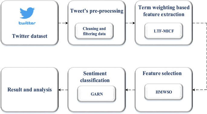
For sentiment classification of Twitter tweets, a DL technique of gated attention recurrent network (GARN) is proposed. The Twitter dataset (Sentiment140 dataset) with sentiment tweets that the public can access is initially collected and given as input. After collecting data, the next stage is pre-processing the tweets. In the pre-processing stage, tokenization, stopwords removal, stemming, slang and acronym correction, removal of numbers, punctuations &symbol removal, removal of uppercase and replacing with lowercase, character &URL, hashtag & user mention removal are done. Now the pre-processed dataset act as input for the next process. Based on term frequency, a term weight is allocated for each term in the dataset using the Log Term Frequency-based Modified Inverse Class Frequency (LTF-MICF) extraction technique. Next, Hybrid Mutation based White Shark Optimizer (HMWSO) is used to select optimal term weight. Finally, the output of HMWSO is fed into the gated attention recurrent network (GARN) for sentiment classification with three different classes. Figure 1 shows a diagrammatic representation of the proposed methodology.

Fig. 1

Architecture diagram

Tweets pre-processing

Pre-processing is converting the long data into short text to perform other processes such as classification, detecting unwanted news, sentiment analysis etc., as Twitter users use different styles to post their tweets. Some may post the tweet in abbreviations, symbols, URLs, hashtags, and punctuations. Also, tweets may consist of emojis, emoticons, or stickers to express the user’s sentiments and feelings. Sometimes the tweets may be in a hybrid form,such as adding abbreviations, symbols and URLs. So these kinds of symbols, abbreviations, and punctuations should be removed from the tweet toclassify the dataset further. The features to be removed from the tweet dataset are tokenization, stopwords removal, stemming, slag and acronym correction, removal of numbers, punctuation and symbol removal, noise removal, URL, hashtags, replacing long characters, upper case to lower case, and lemmatization.

Tokenization

Tokenization [28] is splitting a text cluster into small words, symbols, phrases and other meaningful forms known as tokens. These tokens are considered as input for further processing. Another important use of tokenization is that it can identify meaningful words.The tokenization challenge depends only on the type of language used. For example, in languages such as English and French, some words may be separated by white spaces. Other languages, such as Chinese and Thai words,are not separated. The tokenization process is carried out in the NLTK Python library. In this phase, the data is processed in three forms: convert the text document into word counts. Secondly,data cleansing and filtering occur, andfinally, the document is split into tokens or words.

The example provided below illustrates the original tweet before and after performing tokenization:

Before tokenization

DLis a technology which trains the machineto behave naturally like a human being.

After tokenization

Deep, learning, is, a, technology, which, train, the, machine, to, behave, naturally, like, a, human, being.

Numerous tools are available to tokenize a text document. Some of them are as follows;

• NLTK word tokenize

• Nlpdotnet tokenizer

• TextBlob word tokenize

• Mila tokenizer

• Pattern word tokenize

• MBSP word tokenize

Stopwords removal

Stopword removal [28] is a process of removing frequently used words with meaningless in a text document. Stopwords such as are, this, that, and, so are frequently occurring words in a sentence. These words are also termed pronouns, articles and prepositions. Such words are not used forfurther processing, so removing those words is required. If such words are not removed, the sentence seems heavy and becomes less important for the analyst.Also, they are not considered keywords in Twitter analysis applications. Many methods exist to remove stopwords from a document; they are.

• Z-methods

• Classic method

• Mutual information (MI) method

• Term based random sampling (TBRS) method

Removing stopwords from a pre-compiled list is performed using a classic-based method. Z-methods are known as Zipf’s law-based methods. In Z-methods, three removal processes occur: removing the most frequently used words, removing the words which occur once in a sentence, and removing words with a document frequency of low inverse. In the mutual MI method, the information with low mutual will be removed. In the TBRS method, the words are randomly chosen from the document and given rank for a particular term using the Kullback–Leibler divergence formula, which is represented as;

$$d_{l} (t) = Q_{l} (t).\log_{2} \frac{{Q_{l} (t)}}{Q(t)}$$

(1)

where $Q_{l} (t)$ is the normalized term frequency (NTF) of the term $t$ within a mass $l$, and NTF is denoted as $Q(t)$ of term $t$ in the entire document. Finally, using this equation, the least terms are considered a stopword list from which the duplications are removed.

Stemming

Removing prefixesand suffixes from a word is performed using the stemming method. It can also be defined as detecting the root and stem of a word and removing them. For example, processed word processing can be stemmed from a single word as a process [28]. The two points to be considered while performing stemming are: the words with different meanings must be kept separate, and the words of morphological forms will contain the same meaning and must be mapped with a similar stem. There are stemming algorithms to classify the words. The algorithms are divided into three methods: truncating, statistical, and mixed methods. Truncating method is the process of removing a suffix from a plural word. Some rules must be carried out to remove suffixes from the plurals to convert the plural word into the singular form.

Different stemmer algorithms are used under the truncating method. Some algorithms are Lovins stemmer, porters stemmer, paice and husk stemmer, and Dawson stemmer. Lovins stemmer algorithm is used to remove the lengthy suffix from a word. The drawback of using this stemmer is that it consumes more time to process. Porter’s stemmer algorithm removes suffixes from a word by applying many rules. If the applied rule is satisfied, the suffix is automatically removed. The algorithm consists of 60 rules and is faster than theLovins algorithm. Paice and husk is an iterative algorithm that consists of 120 rules to remove the last character of the suffixed word. This algorithm performs two operations, namely, deletion and replacement. The Dawson algorithm keeps the suffixed words in reverse order by predicting their length and the last character. In statistical methods, some algorithms are used: N-gram stemmer, HMM stemmer, and YASS stemmer. In a mixed process, the inflectional and derivational methods are used.

Slang and acronym correction

Users typically use acronyms and slang to limit the characters in a tweet posted on social media [29]. The use of acronyms and slangis an important issue because the users do not have the same mindset to make the acronym in the same full form, and everyone considers the tweet in different styles or slang. Sometimes, the acronym posted may possess other meanings or be associated with other problems. So, interpreting these kinds of acronyms and replacing them with meaningful words should be done so the machine can easily understand the acronym’s meaning.

An example illustrates the original tweet with acronyms and slang before and after removal.

Before removal: ROM permanently stores information in the system, whereas RAM temporarily stores information in the system.

After removal: Read Only Memory permanently store information in the system, whereas Random Access Memory temporarily store information in the system.

Removal of numbers

Removal of numbers in the Twitter dataset is a process of deleting the occurrence of numbers between any words in a sentence [29].

An example illustrates the original tweet before and after removing numbers.

Before removal: My ink “My Way…No Regrets” Always Make Happiness Your #1 Priority.

After removal: My ink “My Way … No Regrets” Always Make Happiness Your # Priority.

Once removed, the tweet will no longer contain any numbers.

Punctuation and symbol removal

The punctuation and symbols are removed in this stage. Punctuations such as ‘.’, ‘,’, ‘?’, ‘!’, and ‘:’ are removed from the tweet [29, 30].

An example illustrates the original tweet before and after removing punctuation marks.

Before removal: My ink “My Way…No Regrets” Always Make Happiness Your #1 Priority.

After removal: My ink My Way No Regrets Always Make Happiness Your Priority.

After removal, the tweet will not contain any punctuation. Symbol removal is the process of removing all the symbols from the tweet.

An example illustrates the original tweet before and after removing symbols.

Before removal: wednesday addams as a disney princess keeping it .

After removal: wednesday addams as a disney princess keeping it.

After removal, there would not be any symbols in the tweet.

Removal of uppercase into lowercase character

In this process of removal or deletion, all the uppercase charactersare replaced with lowercase characters [30].

An example illustrates the original tweet before and after removing uppercase characters into lowercase characters.

Before removal: My ink “My Way…No Regrets” Always Make Happiness Your #1 Priority.

After removal: my ink my way no regrets always make happiness your priority.

After removal, the tweet will no longer contain capital letters.

URL, hashtag & user mention removal

For clear reference,Twitter users post tweets with various URLs and hashtags [29, 30]. This information ishelpful for the people but mostly noise, which cannot be used for further processes. The example provided below illustrates the original tweet with URL, hashtag and user mention before removal and after removal:

Before removal: This gift is given by #ahearttouchingpersonfor securing @firstrank. Click on the below linkto know more https://tinyurl.com/giftvoucher.

After removal: This is a gift given by a heart touching person for securing first rank. Click on the below link to know more.

Term weighting-based feature extraction

After the pre-processing, the pre-processed data is extracted in text documents based on the term weighting $T_{w}$ [22]. A new term weighting scheme,Log term frequency-based modified inverse class frequency (LTF-MICF), is employed in this research paper for feature extraction based on term weight. The technique integrates two different term weighting schemes: log term frequency (LTF) and modified inverse class frequency (MICF). The frequently occurring terms in the document are known as term frequency $^{f} T$. But, $^{f} T$ alone is insufficient because the frequently occurring terms will possess heavyweight in the document. So, the proposed hybrid feature extraction technique can overcome this issue. Therefore, $^{f} T$ is integrated with MICF, an effective $T_{w}$ approach. Inverse class frequency $^{f} C_{i}$ is the inverse ratio of the total class of terms that occurs on training tweets to the total classes. The algorithm for the TW-FE technique is shown in algorithm 1 [22].

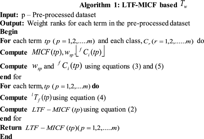
Two steps are involved in calculating LTF $^{l} T_{f}$. The first step is to calculate the $^{f} T$ of each term in the pre-processed dataset. The second step is, applying log normalization to the output of the computed $^{f} T$ data. The modified version of $^{f} C_{i}$, the MICF is calculated for each term in the document. MICF is said to be executed then;each term in the document should have different class-particular ranks, which should possess differing contributions to the total term rank. It is necessary to assign dissimilar weights for dissimilar class-specific ranks. Consequently, the sum of the weights of all class-specific ranks is employed as the total term rank. The proposed formula for $T_{w}$ using LTF-based MICF is represented as follows [22];

$$LTF - MICF(tp) =^{l} T_{f} (tp) * \sum\limits_{r = 1}^{m} {w_{sp} - \left[ {^{f} C_{i} (tp)} \right]}$$

(2)

where a specific weighting factor is denoted $w_{sp}$ for each $tp$ for class $C_{r}$, which can be clearly represented as;

$$w_{sp} = \log (1 + \frac{{s_{i} \mathop{t}\limits^{\rightharpoonup} }}{{\max (1,s_{i} \overleftarrow {t} }}.\frac{{s_{i} \tilde{t}}}{{\max (1,s_{i} \overset{\lower0.5em\hbox{$\smash{\scriptscriptstyle\frown}$}}{t} }}$$

(3)

The method used to assign a weight for a given dataset is known as the weighting factor (WF). Where the number of tweets $s_{i}$ in class $C_{r}$ which contains pre-processed terms $tp$ is denoted as $s_{i} \mathop{t}\limits^{\rightharpoonup}$. The number of $s_{i}$ in other classes, which contains $tp$ is denoted as $s_{i} \mathop{t}\limits^{\leftarrow}$. The number of $s_{i}$ in-class $C_{r}$, which do not possess,$tp$ is denoted as $s_{i} \overset{\lower0.5em\hbox{$\smash{\scriptscriptstyle\frown}$}}{t}$. The number of $s_{i}$ in other classes, which do not possess,$tp$ is denoted as $s_{i} \tilde{t}$. To eliminate negative weights, the constant ‘1’ is used. In extreme cases, to avoid a zero-denominator issue, the minimal denominator is set to ‘1’ if $s_{i} \mathop{t}\limits^{\leftarrow}$ = 0 or $s_{i} \overset{\lower0.5em\hbox{$\smash{\scriptscriptstyle\frown}$}}{t}$ = 0. The formula for $^{l} T_{f} (tp)$ and $^{f} C_{i} (tp)$ can be presented as follows [22];

$$^{l} T_{f} (tp) = \log (1 +^{f} T(tp,s_{i} ))$$

(4)

where raw count of $tp$ on $s_{i}$ is denoted as $^{f} T(tp,s_{i} )$, i.e., the total times of $tp$ occurs on $s_{i}$.

$$^{f} C_{i} (tp) = \log (1 + \frac{r}{C(tp)}$$

(5)

where $r$ refers to the total number of classes in $s_{i}$, and $C(tp)$ is the total number of classes in $tp$. The dataset features are represented as $f_{j} = \left\{ {f_{1} ,f_{2} ,..........f_{3} ,......f_{m} } \right\}$ after $T_{w}$, where the number of weighted terms in the pre-processed dataset is denoted as $f_{1} ,f_{2} ,...f_{3} ,...f_{m}$ respectively. The computed rank values of each term in the text document of tweets are used for performing the further process.

Feature selection

The existence of irrelevant features in the data can reduce the accuracy level of the classification process and make the model to learn those irrelevant features. This issue is termed as the optimization issue. This issue can be ignored only by taking optimal solutions from the processed dataset. Therefore, a feature selection algorithm named White shark optimizer with a hybrid mutation strategy is utilized to achieve a feature selection process.

White Shark Optimizer (WSO)

WSO is proposed based on the behaviour of the white shark while foraging [23]. Great white shark in the ocean catches prey by moving the waves and other features to catch prey kept deep in the ocean. Since the white shark catch prey based on three behaviours, namely: (1) the velocity of the shark in catching the prey, (2) searching for the best optimal food source, (3) the movement of other sharks toward the shark, which is near to the optimal food source. The initial white shark population is represented as;

$$W_{q}^{p} = lb_{q} + r \times (up_{q} - lb_{q} )$$

(6)

where $W_{q}^{p}$ is the initial parameters of the $p_{th}$ white shark in the $q_{th}$ dimension. The upper and lower bounds in the $q_{th}$ dimension are denoted as $up_{q}$ and $lb_{q}$, respectively. Whereas $r$ denotes a random number in the range [0, 1].

The white shark’s velocity is to locate the prey based on the motion of the sea wave is represented as [23];

$$vl_{s + 1}^{p} = \mu \left[ {vl_{s}^{p} + F_{1} (W_{{gbest_{s} }} - W_{s}^{p} ) \times C_{1} + F_{2} (W_{best}^{{vl_{s}^{p} }} - W_{s}^{p} ) \times C_{2} } \right]$$

(7)

where $s = 1,2,....m$ is the index of a white shark with a population size of $m$. The new velocity of $p_{th}$ shark is denoted as $vl_{s + 1}^{p}$ in $(s + 1)_{th}$ step. The initial speed of the $p_{th}$ shark in the $s_{th}$ step is denoted as $vl_{s}^{p}$. The global best position achieved by any $p_{th}$ shark in $s_{th}$ step is denoted as $W_{{gbest_{s} }}$. The initial position of the $p_{th}$ shark in $s_{th}$ step is denoted as $W_{s}^{p}$. The best position of the $p_{th}$ shark and the index vector on attainingthe best position are denoted as $W_{best}^{{vl_{s}^{p} }}$ and $vc^{i}$. Where $C_{1}$ and $C_{2}$ in the equation is defined as the creation of uniform random numbers of the interval [1, 0]. $F_{1}$ and $F_{2}$ are the force of the shark to control the effect of $W_{{gbest_{s} }}$ and $W_{best}^{{vl_{s}^{p} }}$ on $W_{s}^{p}$.$\mu$ represents to analyze the convergence factor of the shark. The index vector of the white shark is represented as;

$$vc = \left[ {t \times rand(1,t)} \right] + 1$$

(8)

where $rand(1,t)$ is a random numbers vector obtained with a uniform distribution in the interval [0, 1].The forces of the shark to control the effect are represented as follows;

$$F_{1} = F_{\max } + (F_{\max } - F_{\min } ) \times e^{{ - (4u/U)^{2} }}$$

(9)

$$F_{2} = F_{\min } + (F_{\max } - F_{\min } ) \times e^{{ - (4u/U)^{2} }}$$

(10)

The initial and maximum sum of the iteration is denoted as $u$ and $U$, whereas the white shark’s current and sub-ordinate velocities are denoted as $F_{\min }$ and $F_{\max }$. The convergence factor is represented as;

$$\mu = \frac{2}{{\left| {2 - \tau - \sqrt {\tau^{2} - 4\tau } } \right|}}$$

(11)

where $\tau$ is defined as the acceleration coefficient. The strategy for updating the position of the white shark is represented as follows;

$$W_{s + 1}^{p} = \left\{ {_{{W_{s}^{p} + vl_{s}^{p} /fr;\,rand\,\, \ge MV}}^{{W_{s}^{p} .\neg \,\, \oplus \,\,W_{ \circ } + up\,\,.\,c + lo\,\,.\,d;\,\,rand < MV}} } \right.$$

(12)

The new position of the $p_{th}$ shark in $(s + 1)$ iteration, $\neg$ represent the negation operator, $c$ and $d$ represents the binary vectors. The search space lower and upper bounds are denoted as $lo$ and $ub$. $W_{0}$ and $fr$ denotes the logical vector and frequency at which the shark moves. The binary and logic vectors are expressed as follows;

$$c = {\text{sgn}} (W_{s}^{p} - up)\,\, > \,0$$

(13)

$$d = {\text{sgn}} (W_{s}^{p} - 1)\,\, > \,\,0$$

(14)

$$W_{o} = \oplus (c,d)$$

(15)

The frequency at which the white shark moves is represented as;

$$fr = fr_{\min } + \frac{{fr_{\max } - fr_{\min } }}{{fr_{\max } - fr_{\min } }}$$

(16)

$fr_{\max }$ and $fr_{\min }$ represents the maximum and minimum frequency rates. The increase in force at each iteration is represented as;

$$MV = \frac{1}{{(c_{0} + e^{{(s/2 - S)/c_{1} }} )}}$$

(17)

where $MV$ represents the weight of the terms in the document.

The best optimal solution is represented as;

$$W_{s + 1}^{\prime p} = W_{{gbest_{s} }} + r_{1} \vec{D}is_{W} {\text{sgn}} (r_{2} - 0.5)r_{3} < Str_{sns}$$

(18)

where the position updation following the food source of $p_{th}$ the white shark is denoted as $W_{s + 1}^{\prime p}$. The ${\text{sgn}} (r_{2} - 0.5)$ produce 1 or −1 to modify the search direction. The food source and shark distance $\vec{D}is_{w}$ and the strength of the white shark following other sharks close to the food source $Str_{sns}$ is formulated as follows;

$$\vec{D}is_{W} = \left| {rand \times (W_{{gbest_{s} }} - W_{s}^{p} } \right|$$

(19)

$$Str_{sns} = \left| {1 - e^{{(c_{2} \times s/S)}} } \right|$$

(20)

The initial best optimal solutions are kept constant, and the position of other sharks is updated according to these two constant optimal solutions. The fish school behaviour of the sharks is formulated as follows;

$$W_{S + 1}^{P} = \frac{{W_{s}^{p} + W_{s + 1}^{\prime p} }}{2 \times rand}$$

(21)

The weight factor $^{j} we$ is represented as;

$$^{p} we = \frac{1}{m - 1} * \left( {\frac{{\sum\limits_{\Upsilon = 1,\Upsilon \ne j}^{\rho } {^{q} fit} }}{{\sum\limits_{\Upsilon = 1}^{\rho } {^{q} fit} }}} \right)$$

(22)

where $^{q} fit$ is defined as the fitness of each term in the text document. The expansion of the equation is represented as;

$$^{p} we = \frac{1}{m - 1} * \frac{{\left[ {^{1} fit +^{2} fit + ....... +^{q + 1} fit + ..... +^{m - 1} fit +^{m} fit} \right]}}{{^{1} fit +^{2} fit + .....^{q - 1} fit +^{q} fit +^{q + 1} fit + .... +^{m - 1} fit +^{m} fit}}$$

(23)

The concatenation of hybrid mutation $HM$ is applied to the WSO for a faster convergence process. Thus, the hybrid mutation applied with the optimizer is represented as;

$$HM =^{t + 1} GM +^{t + 1} CM$$

(24)

$$^{t + 1} GM = W_{q}^{new} + D_{1} .G_{a} (\mu ,\sigma )$$

(25)

$$^{t + 1} CM = W_{q}^{new} + D_{2} .C_{a} (\mu^{\prime},\sigma^{\prime})$$

(26)

whereas $G_{a} (\mu ,\sigma )$ and $C_{a} (\mu ,\sigma )$ represents an arbitrary number of both Gaussian and Cauchy distribution. $(\mu ,\sigma )$ and $(\mu^{\prime},\sigma^{\prime})$ represents the mean and variance function of both Gaussian and Cauchy distributions. $D_{1}$ and $D_{2}$ represents the coefficients of Gaussian $^{t + 1} GM$ along with Cauchy $^{t + 1} CM$ mutation. On applying these two hybrid mutation operators, a new solution is produced that is represented as;

$$[W_{q}^{new} ]_{new} = W_{q}^{new} +^{p} we(HM)$$

(27)

where,

$$p_{we} = \sum {_{y = 1}^{PS} \frac{{W_{q}^{new} }}{PS}}$$

(28)

whereas $^{p}_{we}$ represents the weight vector and $PS$ represents the size of the population. The selected features from the extracted features are represented as $Sel(p = 1,2,...m)$. The WSO output is denoted as $(sel) = \left\{ {sel^{1} ,sel^{2} ,.....sel^{m} } \right.\left. {} \right\}$,which is a new sub-group of terms in the dataset. At the same time,$m$ denotes a new number of each identical feature. Finally, the feature selection stage provides a dataset document with optimal features.

Gated attention recurrent network (GARN) classifier

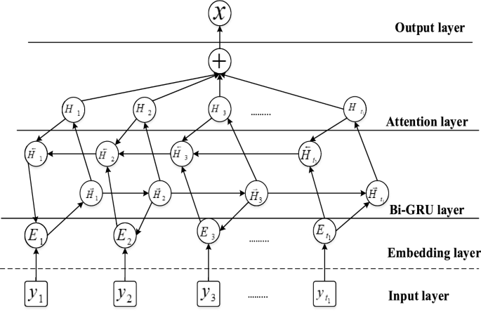
GARN is a hybrid network of Bi-GRU with an attention mechanism. Many problems occur due to the utilization of recurrent neural network (RNNs) because it employs old information rather than the current information for classification. To overcome this problem, a bidirectional recurrent neural network (BRNN) model is proposed, which can utilize both old and current information. So, to perform both the forward and reverse functions, two RNNs are employed. The output will be connected to a similar output layer to record the feature sequence. Based on the BRNN model, another bidirectional gated recurrent unit (Bi-GRU) model is introduced, which replaces the hidden layer of the BRNN with a single GRU memory unit. Here, the hybridization of both Bi-GRU with attention is considered agated attention recurrent network (GARN) [25] and its structure is given in Fig. 2.

Fig. 2

Structure of GARN

Consider an m-dimensional input data as $(y_{1} ,y_{2} ,....,y_{m} )$. The hidden layer in the BGRU produces an output $H_{{t_{1} }}$ at a time interval $t_{1}$ is represented as;

$$\vec{H}_{{t_{1} }} = \sigma \left( {w_{{e\mathop{\longrightarrow}\limits_{{yH}}^{}}} y_{{t_{1} }} + w_{{e\mathop{\longrightarrow}\limits_{H}^{}\mathop{\longrightarrow}\limits_{H}^{}}} \vec{H}_{{t_{1} - 1}} + c_{{\mathop{\longrightarrow}\limits_{H}^{}}} } \right)$$

(29)

$$\overleftarrow {H} _{{t_{1} }} = \sigma \left( {w_{{e_{{\xleftarrow[{yH}]{{}}}} }} y_{{t_{1} }} + w_{{e_{{\xleftarrow[H]{{}}\xleftarrow[H]{{}}}} }} \overleftarrow {H} _{{t_{1} - 1}} + c_{{\xleftarrow[H]{{}}}} } \right)$$

(30)

$$H_{{t_{1} }} = \vec{H}_{{t_{1} }} \oplus \overleftarrow {H} _{{t_{1} }}$$

(31)

where the weight factor for two connecting layers is denoted as $w_{e}$, $c$ is the bias vector, $\sigma$ represents the activation function, positive and negative outputs of GRU is denoted as $\vec{H}_{{t_{1} }}$ and $\overleftarrow {H} _{{t_{1} }}$, $\oplus$ is a bitwise operator.

Attention mechanism

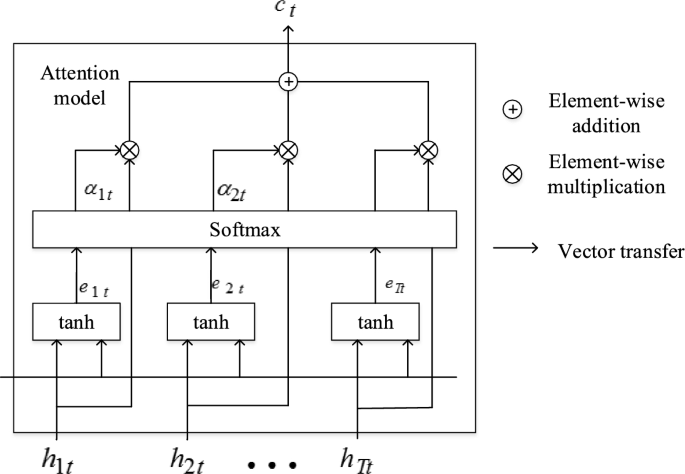
In sentiment analysis, the attention module is very important to denote the correlation between the terms in a sentence and the output [26]. For direct simplification, an attention model is used in this proposal named as feed-forward attention model. This simplification is to produce a single vector $\nu$ from the total sequence represented as;

$$E_{{t_{1} }} = b(H_{{t_{1} }} )$$

(32)

$$\beta_{{t_{1} }} = \frac{{\exp (E_{{t_{1} }} )}}{{\sum\nolimits_{s = 1}^{R} {\exp (E_{s} } )}}$$

(33)

$$\nu = \sum\limits_{{t_{1} = 1}}^{R} {\beta_{{t_{1} }} H_{{t_{1} }} }$$

(34)

Where $\beta$ is a learning function and is identified using $H_{{t_{1} }}$. From the above Eq. 34, the attention mechanism produces a fixed length for the embedding layer in a BGRU model for every single vector $\nu$ by measuring the average weight of the data sequence $H$. The structure for attention mechanism is shown in Fig. 3. Therefore, the final sub-set for the classification is obtained from:

$$H^{\# } = \tanh (\nu )$$

(35)

Fig. 3

Structure of attention mechanism

Sentiment classification

Twitter sentiment analysis is formally a classification problem. The proposed approach classifies the sentiment data into three classes: positive, negative and neutral. For classification, the softmax classifier is used to classify the output in the hidden layer $H^{\# }$ is represented as;

$$Q\left( {x|T} \right) = soft\max \left( {w_{e} H^{\# } + c} \right)$$

(36)

$$x = \arg \mathop {\max }\limits_{x} \,Q\left( {x|T} \right)$$

(37)

where $w_{e}$ is the weight factor, $c$ is a bias vector and $H^{\# }$ is the output of the last hidden layer. Also, the cross-entropy is evaluated as a loss function represented as;

$$loss_{fc} = - \frac{1}{n}\sum\limits_{j = 1}^{n} {sen_{j} \log x_{j} + \lambda ||\theta ||^{2} }$$

(38)

The total number of samples is denoted as, $n$. The real category of the sentence is denoted as $sen_{j}$,the sentence with the predictive category is denoted as $x_{j}$, and the $L2$ regular item is denoted as $\lambda ||\theta ||^{2}$.

Results and discussion

This section briefly describes the performance metrics like accuracy, precision, recall and f-measure. The overall analysis of the Twitter sentiment classification with pre-processing, feature extraction, feature selection and classification are also analyzed and discussed clearly. Results on comparing the existing and trending classifiers with term weighting schemes in bar graphs and tables are included. Finally, a small discussion about the overall workflow concluded the research by importing the analyzed performance metrics. The sentiment is an expression from individuals based on an opinion on any subject. Tweet-based analysis of sentiment mainly focuses on detecting positive and negative sentiments. So, it is necessary to enhance the classification classes in which a neutral class is added to the datasets.

Dataset

The dataset utilized in our proposed work is Sentiment 140, gathered from [27], which contains 1,600,000tweets extracted from Twitter API. The score values for each tweet as, for positive tweets, the rank value is 4.Similarly, for negative tweets rank value is 0, and for neutral tweets, the rank value is 2.The total number of positive tweets in a dataset is 20832, neutral tweets are 18318, negative tweets are 22542, and irrelevant tweets are 12990. From the entire dataset, 70%is used for training, 15% for testing and 15% for validation. Table 2 shows the system configuration of the designed classifier.

Table 2 System configuration of the designed classifier

Performance metrics

In this proposed method, 4 different weight schemes are compared with other existing,proposed classifiers in which the performance metrics are precision, f1-score, recall and accuracy. Four notations, namely, true-positive $(t_{p} )$, true-negative $(t_{n} )$, false-positive $(f_{p} )$ and false-negative, $(f_{n} )$ are particularly utilized to measure the performance metrics.

Accuracy $(A_{c} )$

Accuracy is the dataset’s information accurately being classified by the proposed classifier. The accuracy value for the proposed method is obtained using Eq. 39.

$$A_{c} = \frac{{t_{p} + t_{n} }}{{t_{p} + t_{n} + f_{p} + f_{n} }}$$

(39)

Precision $(P_{r} )$

Precision is defined as the number of terms accurately identified positive to the total identified positively. The precision value for the proposed method is obtained using Eq. 40.

$$P_{r} = \frac{{t_{p} }}{{t_{p} + f_{p} }}$$

(40)

Recall $(R_{e} )$

The recall is defined as the percentage of accurately identified positive observations to the total observations in the dataset. The recall value for the proposed method is obtained using Eq. 41.

$$R_{e} = \frac{{t_{p} }}{{t_{p} + f_{n} }}$$

(41)

F1-score $(F_{s} )$

F1-score is defined as the average weight of recall and precision. The f1-score value for the proposed method is obtained using Eq. 42.

$$F_{s} = 2\frac{{P_{r} .\,\,R_{e} }}{{P_{r} + R_{e} }}$$

(42)

Analysis of Twitter sentiments using GARN

The research paper mainly focuses on classifying Twitter sentiments in the form of three classes, namely, positive, negative and neutral. The data are collected using Twitter api. After collecting data, it is given as input for pre-processing. The unwanted symbols are removed in the pre-processing technique, giving a new pre-processed dataset. Now, the pre-processed dataset is given as an input to extract the required features. These features are extracted from the pre-processed dataset using a novel technique known as the log term frequency-based modified inverse class frequency (LTF-MICF) model, which integrates two-weight schemes, LTF and MICF. Here, the required features are extracted in which the extracted features are given as input to select an optimal feature subset. The optimized feature subset is selected using a hybrid mutation-based white shark optimizer (HMWSO). The mutation is referred to as the Cauchy mutation and the Gaussian mutation. Finally, with the selected feature sub-set as input, the sentiments are classified under three classes using a classifier named gated recurrent attention recurrent network (GARN), which is a hybridization of Bi-GRU with an attention mechanism.

The evaluated value of the proposed GARN is preferred for classifying the sentiments of Twitter tweets. The suggested GARN model is implemented in the Python environment, and the sentiment140 Twitter dataset is utilized for training the proposed model. To evaluate the efficiency of the classifier, the proposed classifier is compared with existing classifiers, namely, CNN (Convolutional neural network), DBN (Deep brief neural network), RNN (Recurrent neural network), and Bi-LSTM (Bi-directional long short term memory). Along with these classifiers, the proposed term weighting scheme (LTF-MICF) with the existing term weighting schemes TF (Term Frequency), TF-IDF (Term-frequency-inverse document frequency), TF-DFS (Term-frequency-distinguishing feature selector), and W2V (Word to vector) are also analyzed. The performance was evaluated for both sentiment classification with an optimizer and without using an optimizer. The metrics evaluated are accuracy, precision, recall and f1-score, respectively.The existing methods implemented and proposed (GARU) are Bi-GRU, RNN, Bi-LSTM, and CNN. The simulation parameters used for processing the proposed and existing methods are discussed in Table 3. This comparative analysis is performed to show the efficiency of a proposed over the other related existing algorithms.

Table 3 Simulation parameters of proposed and existing implemented methods

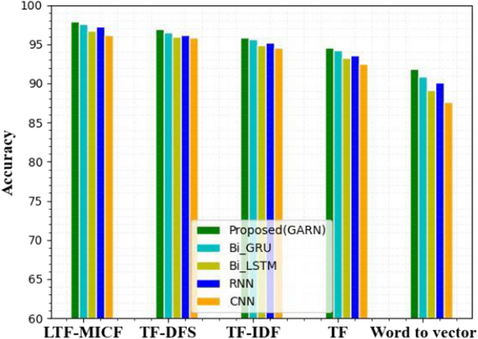
Figure 4 compares the accuracy of the GARN with the existing classifiers. The accuracy obtained by existing Bi-GRU, Bi-LSTM, RNN, and CNN for the LTF-MICF is 96.93%, 95.79%, 94.59% and 91.79%. In contrast, the proposed GARN classifier achieves an accuracy of 97.86% and is considered the best classifier with the LTF-MICF term weight scheme for classifyingTwitter sentiments. But when the proposed classifier is compared with other term weighting schemes,TF-DFS, TF-IDF, TF and W2V, the accuracy obtained is 97.53%, 97.26%, 96.73% and 96.12%. Therefore, the term weight scheme withthe GARN classifier is the best solution for classification problems. Table 4 contains the accuracy values attained by four existing classifiers and the proposed classifier with four existing term weight schemes and proposed term weight scheme.

Fig. 4

Accuracy of the classifiers with term weight schemes

Table 4 Accuracy of the proposed and existing classifiers with term weights

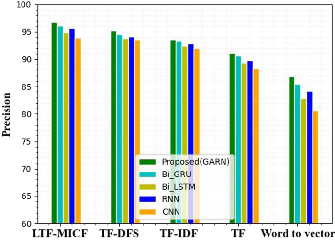
Figure 5 shows the precision performance analysis with the proposed and four existing classifiers for different term weight schemes. The precision of all existing classifiers with other term weight schemes is less than the proposed term weighting scheme. In Bi-GRU, the precision obtained by TF-DFS, TF-IDF, TF and W2V is 94.51%, 94.12%, 93.76% and 93.59%. But, when Bi-GRU is compared with the LTF-MICF term weight scheme, the precision level is increased by 95.22%. The precision achieved by the suggested method GARN with TF-DFS, TF-IDF, TF and W2V is 96.03%, 95.67%, 94.90% and 93.90%. Whereas, when the GARN classifier is compared with the suggested term weighting scheme LTF-MICF the precision achieved is 96.65%, which is considered the best classifier with the best term weighting scheme. Figure 5 shows that the GARN classifier with the LTF-MICF term weighting scheme achieved the highest precision level compared with other classifiers and term weighting schemes.Table 5 indicates the precision performance analysis for existing and proposed classifiers with term weight schemes.

Fig. 5

Precision of the classifiers with term weight schemes

Table 5 Precision of the proposed and existing classifiers with term weights

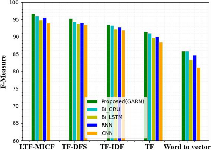
The analysis graph of Fig. 6 shows the f-measure of the four prevalent classifiers and suggested classifiers with different term weight schemes. The f-measure of all the prevalent classifier with other term weight schemes are minimum compared to the suggested term weighting scheme. In Bi-LSTM, the f-measure gained with TF-DFS, TF-IDF, TF and W2V is93.34%, 92.77%, 92.28% and 91.89%. Compared with LTF-MICF, the f-measure level is improved by 95.22%. The f-measure derived by the advance GARN with TF-DFS, TF-IDF, TF and W2V is 96.10%, 95.65%, 94.90% and 94.00%. When GARN is compared with the advanced LTF-MICF scheme, the f-measure grows by 96.70%, which is considered the leading classifier with the supreme term weighting scheme. Therefore, from Fig. 6, the GARN model with the LTF-MICF scheme achieved the greatest f-measure level compared with other DL models and term weighting schemes.Table 6 indicates the performance analysis of the f-measure for both prevalent and suggested classifiers with term weight schemes.

Fig. 6

F-measure of the classifiers with term weight schemes

Table 6 F-measure of the proposed and existing classifiers with term weights

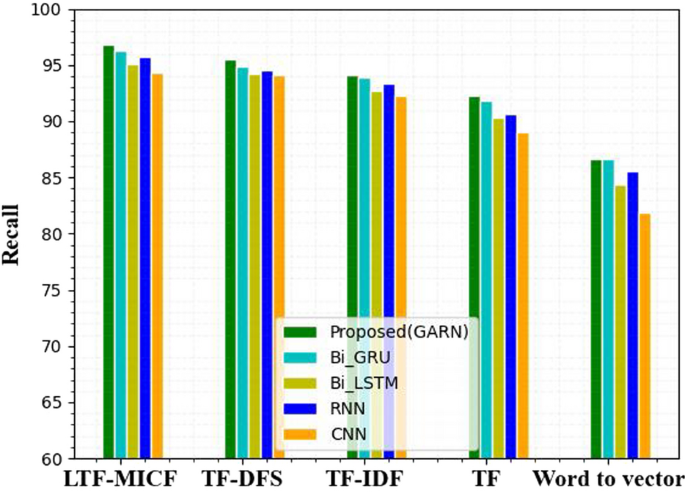
Figure 7 illustrates the recall of the four previously discovered DL models andthe recommended model of dissimilar term weight schemes. The recall of the previously discovered classifier with other term weight schemes is reduced compared to the novel term weighting scheme. In RNN, the recall procured with TF-DFS, TF-IDF, TF and W2V is 91.83%, 90.65%, 90.36% and 89.04%. In comparison with LTF-MICF, the recall value is raised by 92.25%. The recall acquired by the invented GARN with TF-DFS, TF-IDF, TF and W2V is 96.23%, 95.77%, 94.09% and 94.34%. Comparing GARN with the advanced LTF-MICF scheme maximizes recall by 96.76%,which is appraised as the prime classifier with an eminent term weighting scheme. Therefore, from Fig. 7, the GARN model with the LTF-MICF scheme securedextraordinaryrecallvalue when differentiated from other DL models and term weighting schemes. Table 7 indicates the recall performance analysis for the previously discovered and recommended classifiers with term weight schemes.

Fig. 7

Recall of the classifiers with term weight schemes

Table 7 Recall of the proposed and existing classifiers with term weights

Discussion

The four stages employed to implement this proposed work are Twitter data collection, tweet pre-processing, term weighting-based feature extraction, feature selection and classification of sentiments present in the tweet. Initially, the considered tweet sentiment dataset is subjected to pre-processing.Here, tokenization, stemming, punctuations, symbols, numbers, hashtags, and acronyms are removed. After removal, a clean pre-processed dataset is obtained. The performance achieved by proposed and existing methods for solving proposed objective is discussed in Table 8.

Table 8 Performance between proposed and existing methods for developed objective

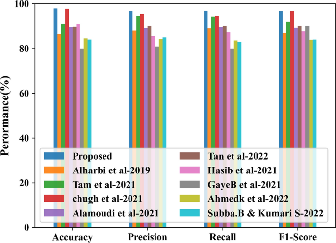
Using this pre-processed dataset, a term weighting-based feature extraction is done using an integrated terms weight scheme such as LTF and MICF as a novel term weighting scheme technique named LTF-MICF technique. An optimization algorithm, HMWSO, with two hybrid mutation techniques, namely Cauchy and Gaussian mutation, is chosen for feature selection. Finally, the GARN classifier is used for the classification of Twitter sentiments. The sentiments are classified as positive, negative and neutral. The performance of existing classifiers with term weighting schemes and the proposed classifier with term weighting schemes are analyzed. The performance comparison between the proposed and existing methods is shown in Table 9. The existing details are collected from previous works developed for sentiment analysis from theTwitter dataset.

Table 9 Performance comparison between developed existing and proposed methods

Many DL techniques use only a single feature extraction technique, namely term frequency (TF) and distinguishing feature selector (DFS), which will not accurately extract the features. The proposed methods without optimization can diminish the proposed model’s accuracy level. The feature extraction technique used in our proposed work will perform greatly because it can extract features from frequently occurring terms in the document. The proposed work uses an optimization algorithm to increase the accuracy level of the designed model.The achieved results are shown in Fig. 8.

Fig. 8

Performance comparison between proposed and existing methods

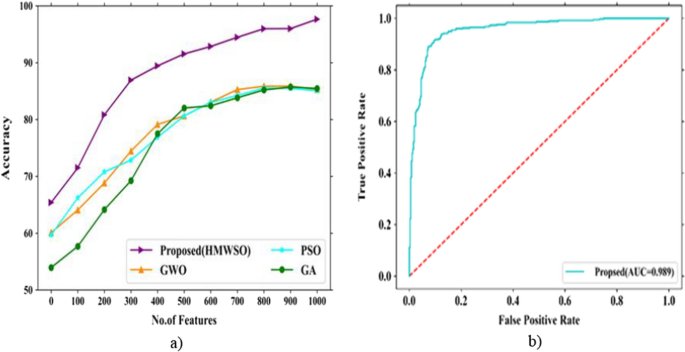
The accuracy comparison by varying the total selected features is described in Fig. 9 (a). The ROC curve of proposed model is discussed in Fig. 9 (b). The ROC is evaluated using FPR (False positive rate), and TPR (True positive rate). The AUC (Area under curve) obtained for proposed is found to be 0.989. It illustrates that the proposed model has shown efficient accuracy with less error rate.

Fig. 9

a Accuracy vs no of features b ROC curve

Ablation study

The ablation study for the proposed model is discussed in Table 10. In this the performance of overall architecture is described, further the comparative analysis between existing techniques also described in Table 10. Among all the techniques the proposed GARN has attained efficient performance than other algorithms. The hybridized methods are separately analysed and the results achieved by such techniques are also analysed which indicates that the integrating of all methods have improved the overall efficiency than applying the techniques in separate manner. Along with that, the ablation study for feature selection process is also evaluated and the obtained results are provided in Table 10.The existing classification and feature selection methods taken for comparison are GRN (Gated recurrent network), ARN (Attention based recurrent network), RNN (Recurrent neural network), WSO, and MO (Mutation optimization).

Table 10 Result analysis related to ablation experiment

The computational complexity of proposed model is defined below:The complexity of attention model is $O\left( {n^{2} \cdot d} \right)$, for recurrent network it is $O\left( {n \cdot d^{2} } \right)$, and the complexity of gated recurrent is found to be $O\left( {k \cdot n \cdot d^{2} } \right)$. The total complexity of proposed GARN is $O\left( {k \cdot n^{2} \cdot d} \right)$. This complexity shows that the proposed model has obtained efficient performance by reducing the system complexity. However, using the model separately won’t provide satisfactory performance. However, integration of such models has attained efficient performance than other existing methods.

Conclusion

GARN is preferred in this research to find the various opinions of Twitter online platform users. The implementation was carried out by utilizing the Sentiment 140 dataset. The performance of the leading GARN classifier is compared with other DL models Bi-GRU, Bi-LSTM, RNN and CNN for four performance metrics: accuracy, precision, f-measure and recall centred with four-term weighting schemes LTF-MICF, TF-DFS, TF-IDF, TF and W2V. The evaluation shows that the leading GARN DL technique reached the target level for Twitter sentiment classification. Additionally, while applying the suggested term weighting scheme-based feature extraction technique LTF-MICF with the leading GARN classifier gained an efficient result for tweet feature extraction. With the Twitter dataset, the GARN accuracy on applying LTF-MICF is 97.86%. The accuracy value attained by the proposed classifier is the highest of all the existing classifiers. Finally, the suggested GARN classifier is regarded as an effective DL classifier for Twitter sentiment analysis and other sentiment analysis applications. The proposed model has attained satisfactory result but it haven’t attained required level. This is because the proposed architecture fails to provide equal importance to the selected features. Due to this, few of the important features get lost, this has reduced the efficient performance of proposed model.Therefore as a future scope, an effective DL technique with the best feature selection method for classifying visual sentiment classification by utilizing all the selected features will be introduced. Further, this method is analysed using the small dataset, therefore in future large data with challenging images will be used to analyse the performance of present architecture.

References

Saberi B, Saad S. Sentiment analysis or opinion mining: a review. Int J Adv Sci Eng Inf Technol. 2017;7(5):1660–6.
Medhat W, Hassan A, Korashy H. Sentiment analysis algorithms and applications: a survey. Ain Shams Eng J. 2014;5(4):1093–113.
Drus Z, Khalid H. Sentiment analysis in social media and its application: systematic literature review. Procedia Comput Sci. 2019;161:707–14.
Zeglen E, Rosendale J. Increasing online information retention: analyzing the effects. J Open Flex Distance Learn. 2018;22(1):22–33.
Qian Yu, Deng X, Ye Q, Ma B, Yuan H. On detecting business event from the headlines and leads of massive online news articles. Inf Process Manage. 2019;56(6): 102086.
Osatuyi B. Information sharing on social media sites. Comput Hum Behav. 2013;29(6):2622–31.
Neubaum, German. Monitoring and expressing opinions on social networking sites–Empirical investigations based on the spiral of silence theory. PhD diss., Dissertation, Duisburg, Essen, Universität Duisburg-Essen, 2016, 2016.
Karami A, Lundy M, Webb F, Dwivedi YK. Twitter and research: a systematic literature review through text mining. IEEE Access. 2020;8:67698–717.
Antonakaki D, Fragopoulou P, Ioannidis S. A survey of Twitter research: data model, graph structure, sentiment analysis and attacks. Expert Syst Appl. 2021;164: 114006.
Birjali M, Kasri M, Beni-Hssane A. A comprehensive survey on sentiment analysis: approaches, challenges and trends. Knowl-Based Syst. 2021;226: 107134.
Yadav N, Kudale O, Rao A, Gupta S, Shitole A. Twitter sentiment analysis using supervised machine learning. Intelligent data communication technologies and internet of things. Singapore: Springer; 2021. p. 631–42.
Jain PK, Pamula R, Srivastava G. A systematic literature review on machine learning applications for consumer sentiment analysis using online reviews. Comput Sci Rev. 2021;41:100413.
Pandian AP. Performance Evaluation and Comparison using Deep Learning Techniques in Sentiment Analysis. Journal of Soft Computing Paradigm (JSCP). 2021;3(02):123–34.
Gandhi UD, Kumar PM, Babu GC, Karthick G. Sentiment analysis on Twitter data by using convolutional neural network (CNN) and long short term memory (LSTM). Wirel Pers Commun. 2021;17:1–10.
Kaur H, Ahsaan SU, Alankar B, Chang V. A proposed sentiment analysis deep learning algorithm for analyzing COVID-19 tweets. Inf Syst Front. 2021;23(6):1417–29.
Alharbi AS, de Doncker E. Twitter sentiment analysis with a deep neural network: an enhanced approach using user behavioral information. Cogn Syst Res. 2019;54:50–61.
Tam S, Said RB, Özgür Tanriöver Ö. A ConvBiLSTM deep learning model-based approach for Twitter sentiment classification. IEEE Access. 2021;9:41283–93.
Chugh A, Sharma VK, Kumar S, Nayyar A, Qureshi B, Bhatia MK, Jain C. Spider monkey crow optimization algorithm with deep learning for sentiment classification and information retrieval. IEEE Access. 2021;9:24249–62.
Alamoudi ES, Alghamdi NS. Sentiment classification and aspect-based sentiment analysis on yelp reviews using deep learning and word embeddings. J Decis Syst. 2021;30(2–3):259–81.
Tan KL, Lee CP, Anbananthen KSM, Lim KM. RoBERTa-LSTM: a hybrid model for sentiment analysis with transformer and recurrent neural network. IEEE Access. 2022;10:21517–25.
Hasib, Khan Md, Md Ahsan Habib, Nurul Akter Towhid, Md Imran Hossain Showrov. A Novel Deep Learning based Sentiment Analysis of Twitter Data for US Airline Service. In 2021 International Conference on Information and Communication Technology for Sustainable Development (ICICT4SD), pp. 450–455. IEEE. 2021.
Zhao H, Liu Z, Yao X, Yang Q. A machine learning-based sentiment analysis of online product reviews with a novel term weighting and feature selection approach. Inf Process Manage. 2021;58(5): 102656.
Braik M, Hammouri A, Atwan J, Al-Betar MA, Awadallah MA. White Shark Optimizer: a novel bio-inspired meta-heuristic algorithm for global optimization problems. Knowl-Based Syst. 2022;243: 108457.
Carvalho F. Guedes, GP. 2020. TF-IDFC-RF: a novel supervised term weighting scheme. arXiv preprint arXiv:2003.07193.
Zeng L, Ren W, Shan L. Attention-based bidirectional gated recurrent unit neural networks for well logs prediction and lithology identification. Neurocomputing. 2020;414:153–71.
Niu Z, Yu Z, Tang W, Wu Q, Reformat M. Wind power forecasting using attention-based gated recurrent unit network. Energy. 2020;196: 117081.
Ahuja R, Chug A, Kohli S, Gupta S, Ahuja P. The impact of features extraction on the sentiment analysis. Procedia Comput Sci. 2019;152:341–8.
Gupta B, Negi M, Vishwakarma K, Rawat G, Badhani P, Tech B. Study of Twitter sentiment analysis using machine learning algorithms on Python. Int J Comput Appl. 2017;165(9):29–34.
Ikram A, Kumar M, Munjal G. Twitter Sentiment Analysis using Machine Learning. In 2022 12th International Conference on Cloud Computing, Data Science & Engineering (Confluence) pp. 629–634. IEEE. 2022.
Gaye B, Zhang D, Wulamu A. A Tweet sentiment classification approach using a hybrid stacked ensemble technique. Information. 2021;12(9):374.
Ahmed K, Nadeem MI, Li D, Zheng Z, Ghadi YY, Assam M, Mohamed HG. Exploiting stacked autoencoders for improved sentiment analysis. Appl Sci. 2022;12(23):12380.
Subba B, Kumari S. A heterogeneous stacking ensemble based sentiment analysis framework using multiple word embeddings. Comput Intell. 2022;38(2):530–59.
Pu X, Yan G, Yu C, Mi X, Yu C. Sentiment analysis of online course evaluation based on a new ensemble deep learning mode: evidence from Chinese. Appl Sci. 2021;11(23):11313.
Chen J, Chen Y, He Y, Xu Y, Zhao S, Zhang Y. A classified feature representation three-way decision model for sentiment analysis. Appl Intell. 2022;1:1–13.
Jain DK, Boyapati P, Venkatesh J, Prakash M. An intelligent cognitive-inspired computing with big data analytics framework for sentiment analysis and classification. Inf Process Manage. 2022;59(1): 102758.
Acknowledgements
Not applicable.
Funding
Authors did not receive any funding for this study.
Author information
Authors and Affiliations
Contributions
NP and PC has found the proposed algorithms and obtained the datasets for the research and explored different methods discussed and contributed to the modification of study objectives and framework. Their rich experience was instrumental in improving our work. BTH and AS has done the literature survey of the paper and contributed writing the paper. All authors contributed to the editing and proofreading. All authors read and approved the final manuscript.
Corresponding author
Ethics declarations
Ethics approval and consent to participate
Consent for publication
Competing interests
The authors declare that they have no Competing interests.
Additional information
Publisher's Note
Springer Nature remains neutral with regard to jurisdictional claims in published maps and institutional affiliations.
Rights and permissions
Open Access This article is licensed under a Creative Commons Attribution 4.0 International License, which permits use, sharing, adaptation, distribution and reproduction in any medium or format, as long as you give appropriate credit to the original author(s) and the source, provide a link to the Creative Commons licence, and indicate if changes were made. The images or other third party material in this article are included in the article's Creative Commons licence, unless indicated otherwise in a credit line to the material. If material is not included in the article's Creative Commons licence and your intended use is not permitted by statutory regulation or exceeds the permitted use, you will need to obtain permission directly from the copyright holder. To view a copy of this licence, visit http://creativecommons.org/licenses/by/4.0/.
About this article
Cite this article
Parveen, N., Chakrabarti, P., Hung, B.T. et al. Twitter sentiment analysis using hybrid gated attention recurrent network. J Big Data 10, 50 (2023). https://doi.org/10.1186/s40537-023-00726-3
Received:
Accepted:
Published:
DOI: https://doi.org/10.1186/s40537-023-00726-3