- Research
- Open access
- Published:
Comparative analysis of deep learning image detection algorithms
Journal of Big Data volume 8, Article number: 66 (2021)
Abstract
A computer views all kinds of visual media as an array of numerical values. As a consequence of this approach, they require image processing algorithms to inspect contents of images. This project compares 3 major image processing algorithms: Single Shot Detection (SSD), Faster Region based Convolutional Neural Networks (Faster R-CNN), and You Only Look Once (YOLO) to find the fastest and most efficient of three. In this comparative analysis, using the Microsoft COCO (Common Object in Context) dataset, the performance of these three algorithms is evaluated and their strengths and limitations are analysed based on parameters such as accuracy, precision and F1 score. From the results of the analysis, it can be concluded that the suitability of any of the algorithms over the other two is dictated to a great extent by the use cases they are applied in. In an identical testing environment, YOLO-v3 outperforms SSD and Faster R-CNN, making it the best of the three algorithms.
Introduction
In recent times, the industrial revolution makes use of computer vision for their work. Automation industries, robotics, medical field, and surveillance sectors make extensive use of deep learning [1]. Deep learning has become the most talked-about technology owing to its results which are mainly acquired in applications involving language processing, object detection and image classification. The market forecast predicts outstanding growth around the coming years. The main reasons cited for this are primarily the accessibility of both strong Graphics Processing Units (GPUs) and many datasets [1]. In recent times, both these requirements are easily available [1].
Image classification and detection are the most important pillars of object detection. There is a plethora of datasets available. Microsoft COCO is one such widely used image classification domain. It is a benchmark dataset for object detection. It introduces a large-scale dataset that is available for image detection and classification [2].
This review article aims to make a comparative analysis of SSD, Faster-RCNN, and YOLO. The first algorithm for the comparison in the current work is SSD which adds layers of several features to the end network and facilitates ease of detection [3]. The Faster R-CNN is a unified, faster, and accurate method of object detection that uses a convolutional neural network. While YOLO was developed by Joseph Redmon that offers end-to-end network [3].
In this paper, by using the Microsoft COCO dataset as a common factor of the analysis and measuring the same metrics across all the implementations mentioned, the respective performances of the three above mentioned algorithms, which use different architectures, have been made comparable to each other. The results obtained by comparing the effectiveness of these algorithms on the same dataset can help gain an insight on the unique attributes of each algorithm, understand how they differ from one another and determine which method of object recognition is most effective for any given scenario.
Literature survey
Object detection has been an important topic of research in recent times. With powerful learning tools available deeper features can be easily detected and studied. This work is an attempt to compile information on various object detection tools and algorithms used by different researchers so that a comparative analysis can be done and meaningful conclusions can be drawn to apply them in object detection. Literature survey serves the purpose of getting an insight regarding our work.
The work done by Ross Girshick has introduced the Fast R-CNN model as a method of object detection [3]. It makes use of the CNN method in the target detection field. The novelty of the method proposed by Girshick has proposed a window extraction algorithm instead of a conventional sliding window extraction procedure in the R-CNN model, there is separate training for the deep convolution network for feature isolation and the support vector machines for categorization [4]. In the fast R- CNN method they have combined feature extraction with classification into a classification framework [3]. The training time is nine times faster in Fast R-CNN than in R-CNN. Whereas in the faster R-CNN method the proposal isolation region and bit of Fast R-CNN are put into a network template referred to as region proposal network (RPN). The accuracy of Fast R-CNN and Faster R-CNN is the same. The research concludes that the method is a combined, deep learning-based object detection system that works at 5–7 fps (Frames Per Second) [4]. Basic knowledge about R-CNN, Fast R-CNN and Faster R-CNN was acquired from this paper. The training of the respective model was also inspired from this paper.
Another research work done by Kim et al is discussed here. This research work uses CNN with background subtraction to build a framework that detects and recognizes moving objects using CCTV (Closed Circuit Television) cameras. It is based on the application of the background subtraction algorithm applied to each frame [5]. An architecture similar to the one in this paper was used in our work.
Another detection network is YOLO. Joseph Redmon et al have proposed You Only Look Once (YOLO)—A one-time convolutional neural network for the prediction of the frame position and classification of multiple candidates is offered by YOLO. End-to-end target detection can be achieved this way. It uses a regression problem to solve object detection. A single end-to-end system completes the process of putting the output obtained from the original image to the category and position [6]. Bounding box prediction and feature extraction of YOLO architecture in our work was inspired by the technique discussed in this paper.
Tanvir Ahmed et al have proposed a modified method that uses an advanced YOLO v1 network model which optimizes the loss of function in YOLO v1, it has a new inception model structure, has a specialized pooling pyramid layer, and has better performance. The advanced application of YOLO is taken from this research paper. It is also an end-to-end process that carries out an extensive experiment on a PASCAL VOC (Visual Object Classes) dataset. The network is an improved version and also shows high effectiveness [7]. The training of the YOLO model using PASCAL VOC was done using the technique proposed in this paper.
Wei Liu et al came up with a new method of detecting objects in images using a single deep neural network. They named this procedure the Single Shot MultiBox Detector SSD. According to the team, SSD is a simple method and requires an object proposal as it is based on the complete elimination of the process that generates a proposal. It also eliminates the subsequent pixel and resampling stages. So, it combines everything into a single step. SSD is also very easy to train and is very straightforward when it comes to integrating it into the system. This makes detection easier. The primary feature of SSD is using multiscale convolutional bounding box outputs that are attached to several feature maps [8]. Training and model analysis of the SSD model of our work was inspired by the work discussed here.
Another paper is based on an advanced type of SSD. In his paper, the authors have proposed their research work to introduce Tiny SSD, a single shot detection deep convolutional neural network. TINY SSD aimed to ease real-time embedded object detection. It comprises of greatly enhanced layers comprising of non-uniform Fire subnetwork and a stack of non-uniform subnetwork of SSD based auxiliary convolutional feature layers. The best feature of Tiny SSD is its size of 2.3 MB which is even smaller than Tiny YOLO. The results of this work have shown that Tiny SSD is well suited for embedded detections [9]. A similar model of SSD was used for the purpose of comparison.
The paper by Pathak et al describes the role of deep learning technique by using CNN for object detection. The paper also accesses some deep learning techniques for object detection systems. The current paper states that deep CNNs work on the principle of weight sharing. It gives us information about some crucial points in CNN.
These features of CNN depicted in this paper are: [1]
-
a.
CNN is integration and involves the multiplication of two overlapping functions.
-
b.
Features maps are abstracted to reduce their complexity in terms of space
-
c.
Repetition of the process is done to produce the feature maps using filters.
-
d.
CNN utilizes different types of pooling layers.
This paper was used as the basis for understanding Convolutional Neural Networks and their role in deed learning.
In a recent research work by Chen et al, they have used anchor boxes for face detection and more exact regression loss function. They have proposed a face detector termed as YOLO face which is based on YOLOv3 that aims at resolving detection problems of varying face scales. The authors concluded that their algorithm out performed previous YOLO versions and its varieties [10]. The YOLOv3 was used in our work for comparison with other models.
In the research work by Fan et al, they have proposed an improved system for the detection of pedestrians based on SSD model of object detection. In this work the multi-layered system they introduced the Squeeze-and-Excitation model as an additional layer to the SSD model. The improved model employed self-learning that further enhanced the accuracy of the system for small scale pedestrian detection. Experiments on the INRIA dataset showed high accuracy [11]. This paper was used for the purpose of understanding the SSD model.
In a recent survey published by Mittal et al, they discussed the algorithms namely Faster RCNN, Cascade RCNN, R-FCN, YOLO and its variants, SSD, RetinaNet and CornerNet, Objects as Point under advanced phases in detectors based on deep learning. This paper provides a comprehensive summary of low-altitude datasets and the algorithms used for the respective work [12]. Our comparison work was done using coco metrics similar to the comparison that has been done in this paper. The paper also discusses several other techniques for comparison which were considered in our work.
Background
Artificial Intelligence (AI): It is a system's ability to correctly interpret external data, to learn from such data, and to use those learnings to achieve specific goals and tasks through flexible adaptation [13].
Machine Learning (ML): It is the study of algorithms that improve automatically through experience [14]. ML algorithms build a training model based on sample data, and using it, make predictions or decisions without being ‘explicitly programmed to do so’.
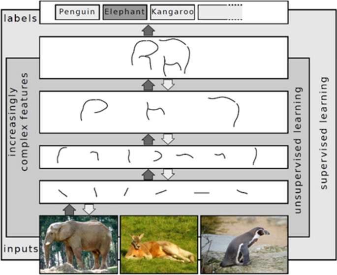
Deep Learning (DL): It is the most used and most preferred approach to machine learning. It is inspired by the working of the biological brain—how individual neurons firing on receiving input only see a very small part of the total input/processed data. It has multiple layers. Upper layers build on the outputs from lower layers. Thus, the higher the layer, the more complex is the data it processes [15].
Identify more complex patterns—animals, faces, objects, skies, etc. A CNN consists of alternating convolutional and pooling layers with at least one fully connected layer at the end.
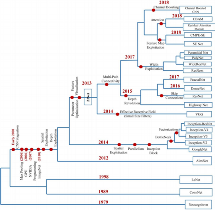
Evolution of CNNs
Convolutional Neural Network (CNN): It is a type of artificial neural network that is mainly used to analyse images. It was inspired by the neurological experiments conducted by Hubel and Wiesel on the visual cortex [17]. The visual cortex is the primary region processing visual sensory information in the brain. It extracts features from images and detects patterns and structures to detect objects in the images. Its distinct feature is the presence of convolutional layers that are hidden. These layers apply filters to extract patterns from images. The filter moves over the image to generates the output. Different filters recognize different patterns. Initial layers have filters to recognize simple patterns. They become more complex through the layers over time as follows:
-
1.
Origin (Late 1980s–1990s): The first popular CNN was LeNet-5 developed in 1998 by LeCun et al. [18]. It was in development for almost a decade. Its purpose was to detect handwritten digits. It is credited for sparking R&D of efficient CNNs in the field of deep learning. Banks started using it in ATMs.
-
2.
Stagnation (Early 2000s): The internal working of CNNs was not yet understood during this period. Also, there was no dataset of a variety of images like Google’s Open Images or Microsoft’s COCO. Hence, most CNNs were only focused on optical character recognition (OCR). CNNs also required high computational time; increasing operating cost. Support Vector Machine (SVM), a machine learning model was showing better results than CNN.
-
3.
Revival (2006–2011): Ranzato et al. in their paper demonstrated that using the max-pooling algorithm for feature extraction instead of the sub-sampling algorithm used earlier results in significant improvement [19]. Researchers had started using GPUs to accelerate training of CNNs. Around the same time, NVIDIA introduced the CUDA platform that allowed and facilitated parallel processing, thus speeding up CNN training and validation [20]. This re-sparked research. In 2010, Stanford University established a large image dataset called Pattern Analysis, Statistical modelling and Computational Learning Visual Object Classes (PASCAL VOC), removing yet another hurdle.
-
4.
Rise (2012–2013): AlexNet was a major breakthrough for accuracy of CNNs. It achieved an error rate of just 15.3% in the 2012 ILSVR challenge. The second-place network had an error rate of 26.2% [21]. So, AlexNet was better by a large margin of 10.8% than any other network known at the time. AlexNet achieved this accuracy by having a total of 8 layers [21], thus truly realizing ‘deep’ learning. This required greater computational power, but the advances in GPU technology made it possible. AlexNet, like LeNet is one of the most influential papers to ever be published on CNNs.
-
5.
Architectural Innovations (2014–2020): The well-known and widely used VGG architecture was developed in 2014 [22]. RCNN, based on VGG like many others, introduced the idea that objects are located in certain regions of the image; hence the name: region-based CNN [23]. Improved versions of RCNN—Fast RCNN [24] and Faster RCNN [3] came out in the subsequent years. Both of these reduced computation time, while maintaining the accuracy that RCNN is known for. Single Shot Multibox Detector (SSD), also based on VGG was developed around 2016 [8]. Another algorithm, You Only Look Once (YOLO), based on an architecture called DarkNet was first published in 2016 [6]. It is in active development; its third version was released in 2018 [25].
Existing methodologies
SSD
Other object detection models such as YOLO or Faster R-CNN perform their operations at a much lesser speed as compared to SSD, making a much more favourable object detection method.
Before the development of SSD, several attempts had been made to design a faster detector by modifying each stage of the detection pipeline. However, any significant increase in speed by such modifications only resulted in a decrease in the detection’s accuracy and hence researchers concluded that rather than altering an existing model, they would have to come up with a fundamentally different object detection model, and hence, the creation of the SSD model [8].
SSD does not resample pixels or features for bounding box hypotheses and is as accurate as models that do. In addition to this, it is quite straightforward compared to methods that require object proposals because it completely eradicates feature resampling stages or pixel and proposal generation, by encompassing all computation in a single network. Therefore, SSD is very simple to train and can be easily integrated into systems that perform detection as one of their functions [8].
It’s architecture heavily depends on the generation of bounding boxes and the extraction of feature maps, which are also known as default bounding boxes. Loss is calculated by the network, using comparisons of the offsets of the predicted classes and the default bounding boxes with the training samples’ ground truth values, using different filters for every iteration. Using the back-propagation algorithm and the calculated loss value, all the parameters are updated. This way, SSD is able to learn the most optimal filter structures that can accurately identify the object features and generalize the given training samples in order to minimize the loss value, resulting in high accuracy during the evaluation phase [26].
Analysis of the functions
SSD is built on a feed-forward complex network that builds a collection of standard-size bounding boxes and for each occurrence of an object in those boxes, a respective score. After score generation, non-maximum suppression is used to generate the final detection results. The preliminary network layers are built on a standard architecture utilized for high quality image classification (and truncated before any classification layers), which is a VGG-16 network. An auxiliary structure is added to the truncated base network such as convo6 to produce detections.
-
1.
Extracting feature maps: SSD uses the VGG-16 architecture to extract feature maps because it shows very good performance for the classification of images with high quality. The reason for using auxiliary layers is because they allow us to extract the required features at multiple scales as well as reduce the size of our input with each layer that is traversed through [8]. For each cell in the image, the layer makes a certain number of predications. Each prediction consists of a boundary box and the box generates scores for all the classes it detects in this box including a score for no object at all. It is an algorithm making a ‘guess’ as to what is in the boundary box by choosing the class with the highest score. These scores a called ‘confidence scores’ and making such predictions is called ‘MultiBox’. Figure 1 depicts the SSD model with the extra feature layers.
-
2.
Convolutional predictors for object detection: Every feature layer produces a fixed number of predictions by utilising convolutional filters. For every feature layer of size x × y having n channels, the rudimentary component for generating prediction variables of a potential detection result is a 3 × 3 × x small kernel that creates a confidence score for every class, or a shape offset calculated with respect to the default grounding box coordinates which are provided by the COCO Dataset at every single one of the ‘x x y’ locations [8].
-
3.
Default boxes and aspect ratios: By now, you may be able to infer that every single feature map cell is associated with a corresponding default bounding box for multiple feature maps in the network. The default boxes are responsible for determining the feature map in a complex manner so that the placement of each box concerning its corresponding cell is fixed. At each feature map cell, we speculate the offsets concerning the default box shapes in the cell and the scores for each class which tells us about the class of object present inside the bounding box. Going into further detail, for every box out of b at a particular given location, s class scores are calculated and its 4 offsets relative to the primal default box shape. This computation results in a total of (s + 4) b filters that are applicable to every location in the feature map, resulting in (s + 4) × b × x × y outputs for a x × y feature map. [8]
Deep Learning Layers illustration [15]
SSD Training Process
-
1.
Matching Process: All SSD predictions are divided into two types; negative matches or positive matches. Positive matches are only used by SSD to calculate the localization cost which is the misalignment of the boundary box with the default box. The match is positive only if the corresponding default boundary box’s IoU is greater than 0.5 with the ground truth. In any other case, it is negative. IoU stands for the ‘intersection over the union’. It is the ratio between the intersected area over the joined area for two regions. IoU is also referred to as the Jaccard index and using this condition makes the learning process much easier [8].
-
2.
Hard negative mining: After the matching step, almost all of the default boxes are negatives, largely when the total count of possible default boxes is high. This causes a large imbalance between the positive and negative training examples. Rather than using up all the negative examples, SSD sorts them by their greatest confidence loss for each default box, the highest ones such that at any point of time, the ratio of the positives and negatives is a maximum of 3:1. This leads to faster optimization and better training [8].
-
3.
Data augmentation: This is crucial for increasing accuracy. There are several data augmentation techniques that we may employ such as color distortion, flipping, and cropping. To deal with a variety of different object sizes and shapes, each training image is randomly picked using one of the methods listed below: [8].
-
We use the original,
-
Sample a patch with IoU of 0.1, 0.3, 0.5, 0.7 or 0.9,
-
Sample a patch randomly.
-
-
4.
Final detection: The results are generated by performing NMS on multi-scale refined bounding boxes. Using the above-mentioned methods such as hard negative mining, data augmentation, and a larger number of other methods, SSD’s performance is much greater than that of Faster R-CNN when it comes to accuracy on PASCAL VOC dataset and the COCO dataset, while being three times faster [26]. The SSD300, where the size of the input image is 300_300, runs at 59 FPS, which is much more efficient and accurate than YOLO. However, SSD is not as efficient at detection for smaller objects, which can be solved by having a more efficient feature extractor backbone (e.g., ResNet101), with the addition of deconvolution layers along with skip connections to create additional large-scale context, and design a better network structure [27].
Complexity analysis
For most algorithms,time-complexity is dependent on the size of input and can be defined in terms of the big-Oh notation. However,for deep-learning models, time complexity is evaluated in terms of the total time taken by SSD to be trained and the inference time when the model is run on specific hardware (Fig. 2).
Evolution of CNNs from 1979 through 2018 [16]
Deep learning models are required to carry out millions of calculations which can prove to be quite expensive computationally, however most of these calculations end up being performed parallelly by the thousands of identical neurons in each layer of the artificial neural network. Due to this parallel nature , it has been observed that training an SSD model in a Nvidia GeForce GTX 1070i GPU reduces the training time by a factor of ten [28].
When it comes to time-complexity, matrix multiplication in the forward pass of the base CNN takes up the most amount of time. The total number of multiplications is dependent on the number of layers in the CNN along with more specific details such as the number of neurons per layer, the amount of filters along with their respective sizes, the size of the feature extraction map and the image’s resolution. The activation function used at each layer is a ReLu function that has been found to run in quadratic time for each neuron in each layer. Hence, taking all these factors into account, we can determine the time-complexity of the forward pass at the base CNN :
Here, b denotes the index of the CNN layer, B is the total amount of CNN layers,xb is the number of filters in the bth layer,h is the filter width and height, xc is the number of neurons, xb-1 is the total number of input channels of the bth layer, sb is the size of the output feature map.
It should be noted that five to ten percent of the training time is taken up by things like dropout,regression,batch normalisation,classification as well.
As for SSD’s accuracy, it is determined by Mean Average Precision or mAP which is simply the average of APs over all classes from the area under the precision-recall curve. A higher mAP is an indication of a more accurate model [28].
Faster R-CNN
R-CNN stands for Region-based Convolutional Neural Networks. This method combines region proposals for object segmentation and high capacity CNNs for object detection [28].
The algorithm of the original R-CNN technique is as follows: [29]
-
1.
Using a Selective Search Algorithm, several candidate region proposals are extracted from the input image. In this algorithm, numerous candidate regions are generated in initial sub-segmentation. Then, regions which are similar are combined to form bigger regions using a greedy algorithm. These regions make up the final region proposals.
-
2.
The CNN component warps the proposals and extracts distinct features as a vector output.
-
3.
The features which are extracted are fed into an SVM (Support Vector Machine) for recognizing objects of interest in the proposal.
Figure 4 given below explains the features and working of R-CNN.
This technique was plagued by a lot of drawbacks. The requirement to classify ~2000 region proposals make the training of the CNN a very time-consuming process. This makes real-time implementation impossible as each test image would take close to 47 seconds for execution.
Furthermore, machine learning could not take place as the Selective Search Algorithm is a fixed algorithm. This could result in non-ideal candidate region proposals being generated [29].
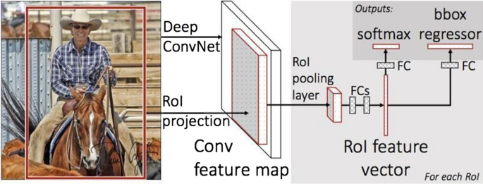
Fast R-CNN is an algorithm for object detection that solves some of the drawbacks of R-CNN. It uses an approach similar to that of its predecessor, but as opposed to using region proposals, the CNN utilizes the image itself for creating a convolutional feature map, following which region proposals are determined and warped from it. An RoI (Region of Interest) pooling layer is employed for reshaping the warped squares according to a predefined size for a fully connected layer to accept them. The region class is then predicted from the RoI vector with the help of a SoftMax layer [24].
Fast R-CNN is faster than its predecessor because feeding ~2000 proposals as input to the CNN per execution is not required. The convolution operation is done to generate a feature map only once per image. [24] The Fig. 3 given below describes the features and working of Fast RCNN.
SSD model [8]
This algorithm shows a significant reduction in time required for both training and testing when compared to R-CNN. But it was noticed that including region proposals significantly bottlenecks the algorithm, reducing its performance [3].
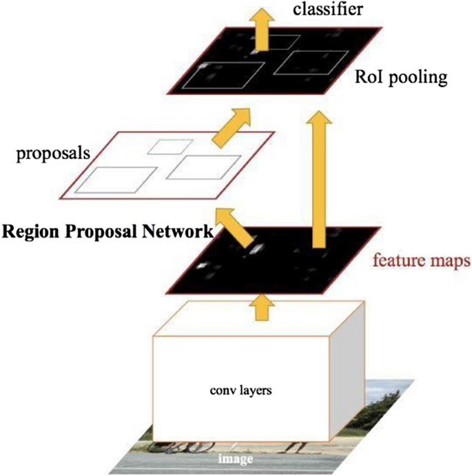
Both Fast R-CNN and its predecessor used Selective Search as the algorithm for determining the region proposals. This being a very time-sapping algorithm, Faster R-CNN eliminated the need for its implementation and instead let the proposals be learned by the network. Just as in the case of Fast R-CNN, a convolutional map is obtained from the image. But a separate network replaces the Selective Search algorithm to predict proposals. These proposals are then reshaped and classified using RoI (Region of Interest) pooling. Refer to the Fig. 4 for the working of Faster R-CNN.
R-CNN model [15]
Faster R-CNN offers an improvement over its predecessors so significant that it is now capable of being implemented for real-time object detection.
Architecture of faster R-CNN
The original implementation of Faster Region-based Convolutional Neural Network (Faster R-CNN) algorithm was experimented on two architectures of convolutional networks: The ZF (Zeiler and Fergus) model, with 5 convolutional layers that a Fast R-CNN network shares with it; and the VGG-16(Simonyan and Zisserman) model, with 13 convolutional layers shared [3] .
The ZF model is based on an earlier model of a Convolutional Network (made by Krizhevsky, Sutskever and Hinton) [30] . This model consisted of eight layers, of which five were convolutional and the remaining three were fully connected [21] .
This architecture exhibited quite a few problems. The first layer filters had negligible coverage medium frequency information compared to that of the very extremes, and the large stride 4 used in the first layer caused aliasing artifacts in the second layer. The ZF model fixed these issues by reducing the size of the first and second layer and making the convolution stride 2, allowing it to hold more information in the first and second layers, and improve classification performance [30] .
Complexity analysis
Region based Convolutional Neural Network (RCNN) and Fast-RCNN both use Selective Search. Selective Search is a greedy algorithm. Greedy algorithms don’t always return the best result [31]. Also, it needs to run multiple times. However, RCNN runs selective search about 2000 times on the image. Fast-RCNN extracts all the regions first and runs selective search just once. This way it reduces time complexity by a large factor [3]. Faster RCNN (FRCNN) removes the final bottleneck—Selective Search. It does so by instead using the Region Proposal Network (RPN). RPN fixes the regions as a grid of n × n. It needs to run fewer number of times as compared to selective search [3] .
As shown in the diagram above, FRCNN consists of Deep Fully Convolutional Network (DFCN), Region Proposal Network, ROI pooling, Fully Connected (FC) networks, Bounding Box Regressor and Classifier.
We will consider DFCN to be ZF-5 for consistent calculation [30]. First feature map, M of dimensions 256 × n × n is extracted from input image, P [33]. Then it is fed to RPN and ROI.
RPN: There are ‘k’ anchors for each point on M. Hence, Total anchors = n × n × k. Anchors are ranked according to score; 2000 anchors are obtained through Non-Maximum Suppression [3]. The Complexity comes out to be O(N2/2).
ROI: Anchors get divided into H × W grid of sub-windows based on M. Output grid is obtained by max-pooling values in corresponding sub-windows. ROI is special case of spatial pyramid pooling layer used in SPP-net, with just one pyramid layer [24]. Hence, complexity becomes O(1).
YOLOv3
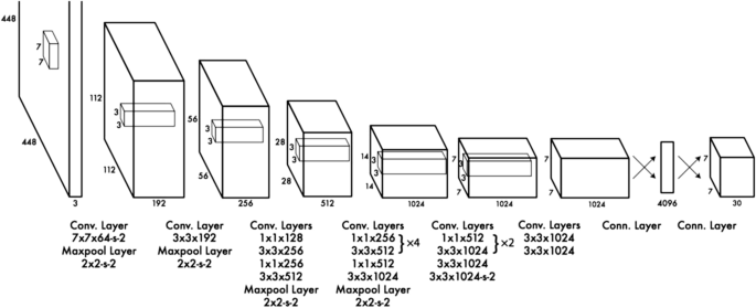
In modern times YOLO (You Only Look Once) is one of the most precise and accurate object detection algorithms available. It has been made on the basis of a newly altered and customized architecture named Darknet [25]. The first version was inspired by Google Net, which used tensor to sample down the image and predicted it with the maximum accuracy. The tensor is generated on the basis of a similar procedure and structure which is also seen in the Region of Interest that is pooled and compiled to decrease the number of individual computations and make the analysis swifter) that is used in the Faster R-CNN network. The following generation utilized an architecture with just 30 convolutional layers, that in turn consisted of 19 layers from DarkNet-19 and an extra 11 for detection of natural objects or objects in natural context as the COCO dataset and metrics have been used. It provided more precise detection and with good speed, although it struggled with pictures of small objects and small pixels. But version 3 has been the greatest and most accurate version of YOLO which has been used widely because of its high precision. Also, the architecture with multiple layers has made the detection more precise [26].
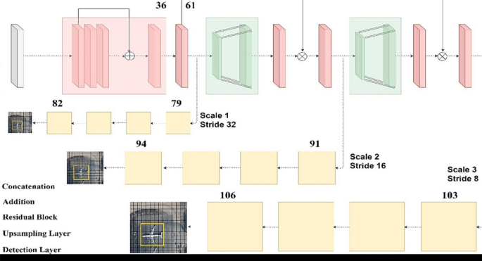
YOLOv3 makes use of the latest darknet features like 53 layers and it has undergone training with one of the most reliable datasets called ImageNet. The layers used are from an architecture Darnnet-53 which is convolutional in nature. For detection, the aforementioned 53 layers were supplemented instead of the pre-existing 19 and this enhanced architecture was trained and instructed with PASCAL VOC. After so many additional layers the architecture maintains one of the best response times with the accuracy offered. It also is very helpful in analysing live video feed because of its swift data unsampling and object detection techniques. One can notice that this version is the best enhancements in ML (Machine Learning) using neural networks. The previous version did not work well with the images of small pixels but the recent updates in v3 have made it very useful in analysing satellite imaging even for defence departments of some countries. The architecture performs in 3 different layers which makes it more efficient but the process is a little slower yet state-of-the-art. For understanding, the framework refers to the Fig. 5 given below.
Fast R-CNN [16]
Feature extraction and analysis [34]
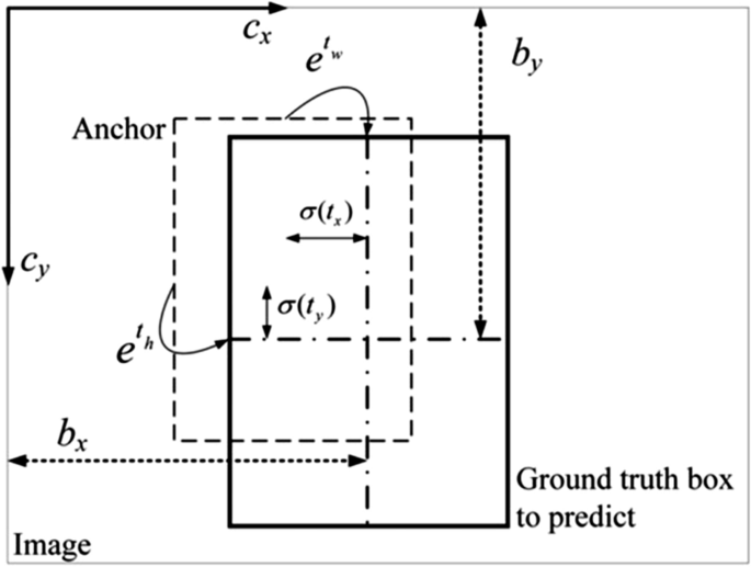
1. Forecasting: This model utilizes packages of different lengths and breadths to produce the weights and frames that establish a strong foundation. This technique is an individual where the network determines the objectivity and allocation independently. The logical regression is used by YOLOv3 where it foresees the objectivity score. It is projected over the selection frame initially on the object that has been established to be the fundamental truth in the picture by pre-training models [35]. This gives a singular bounding box and any kind of fallacy in this part would cause mistakes in both allocation of these boxes and their accuracy and also in the detection arrear. The bounding box forecasting is depicted in the equation given below and Fig. 6.
Faster R-CNN [3]
Equations for bounding box forecasting [34]
2. Class Prediction: YOLOv3 executes a soft-max function to alter the scores to an understandable format for the code. The format is 1. YOLOv3 uses multiple classifications by tag. These tags are custom and non-exclusive. For eg. ‘man’ and ‘woman’ are not exclusive. The architecture modifies the function with individualistic logistic classifiers. YOLOv3 uses binary loss function initially. It uses the soft-max function after that. This leads to a reduction in complexity by avoiding it for the first implementation [36].
3. Predictions: Three distinct orders and dimensions are used for pre-determining the bounding boxes. These are in combination with the function extractor, DarkNet-53. The last levels include detection and categorization into object classes. 3 takes are what is taken on each scale of the COCO dataset. That leads to more than 70 class predictions as an o/p tensor. These features are a classic coder-decoder design introduced in Single-Shot-Detector. The grouping of k-means is also used for finding the best bounding boxes. Finally, in the COCO dataset dimensions like 10 × 13, 62 × 45 and others are used. In total there are 9 distinct dimensions including the aforementioned.
4. DarkNet-53 - The feature Extractor: YOLOv2 had the implementation of DarkNet-19 but in the recently modified model of YOLO Darknet-53 is being used where the 53 is 53 convolutional levels. Speed and accuracy both are an enhanced in Darknet 53 making it 1.5 times quicker. When this architecture is put to compete with ResNet-152, it almost the same performance in terms of accuracy and precision but it is twice as fast [37]. The following Fig. 7 shows the YOLO model.
CNN of the Krizhevsky model [21]
Complexity analysis
The YOLO network is based on a systematic division of the given image into grid. The grids are of 3 types which will be mentioned later. These grids serve as a separate image for the algorithm and they undergo further divisions. YOLO utilizes boundaries that are called bounding boxes. These are the anchors for the analysis of an image. These boxes are essentially acknowledged as resulted even though thousands and thousands are ignored because of the low probability scores and are treated as false positives. These boxes are the manifestation of the rigorous breaking down of an image into grids of cells [38,39,40].
For determining suitable anchor box sizes, YOLO uses K-means clustering to clutch the boxes among the training data. These prior boxes are the guidelines for the algorithm. After receiving the aforementioned data, the algorithm looks for objects with symmetrical shape and size. YOLO uses 3 boxes as anchor so each grid cell puts out 3 boxes. The further predictions and analysis are based on these 3 anchor boxes. Some cases and studies involve the use of 2 anchor box leading to 2 boxes per grid cell [39].
In the above Fig. 8, we can see the anchor box as the dashed box and the forecast of the ground truth or the bounding box is the box with the highlighted borders. There are multiple examples of sizes of image floating around. Each have a distinctive grid cell size and shape. For our model we have taken the standard 448 × 448 image size. The other sizes used for analysis are 416 × 416, 608 × 608 etc. and the grid sizes for them are 19 × 19, 38 × 38 & 76 ×76 and 13 × 13, 52 × 52 & 26 × 26 respectively [40, 41].
Bounding box forecasting [34]
For the first step, the image is modified and altered to a size of 448 x 448 and then the image is put through a slice and dice system where they are divided into 7 x 7 size. This implies that the size of each grid is of size 64 x 64. Every single one of these grid cells produce a certain number of bounding boxes. It may vary from version to version (multiple versions in YOLOv3). For our model we are using 2 boxes per grid. This gives us 4 coordinates per bounding box. They are xcenter, ycenter, width, height. Also, there’s a corresponding confidence value [32].
Use of K-means clustering algorithm gives exponential time complexity O(nkd) where k is the number of images and d is the dimension of the images. After a thorough and stable optimisation technique, the creators have made YOLOv3 the fastest image detection algorithm among the ones mentioned in the paper.
Dataset
MICROSOFT COCO
In recent times for the search of a perfect combination of algorithm and data set, contenders have used the top and highly rated deep learning architectures and data sets. They are used for arriving at the best possible precision and accuracy. The most commonly used data sets are PASCAL VOC and Microsoft COCO. For the review analysis, COCO is used as a dataset and an evaluation metric. They applied different ways of analysis, tweaking and calibrating the base networks and adjusting the software; that leads to better precision but also for improving accuracy, speed, and local split performance [26].
For Object detection, the use of computationally costly architectures and algorithms such as RCNN, SPP-NET (Spatial Pyramid Pooling Network) the use of smart data sets having varied objects and images which also have various objects and are of different dimensions have become a necessity. Not to forget the extreme scope in live video feed monitoring the cost of detection becomes too high. Recently the advancement in deep learning architectures has lead algorithms like YOLO and SSD networks to detect objects by the access to a singular NN (neural network). The introduction of latest architectures has increased the competition between various techniques [26]. But recently COCO has emerged as the most used data set for training and classification. Also, more developments have made it alterable for adding classes [2].
Furthermore, COCO is better than other popular widely used data sets as per some research papers [2]. They are namely Pattern Analysis, Statistical Modelling and Computational Learning Visual Object Classes, ImageNet & SUN (Scene Understanding). The above-mentioned data sets vary hugely based on size, categories, and types. ImageNet was made to target a wider category where the number of different categories but they were fine-grained. SUN focused on more of a modular approach where the regions of interest were based on the frequency of them occurring in the data set. Finally, PASCAL VOC’s was similar yet different in approach to COCO. It used a wide range of images taken from the environment and nature. Microsoft Common Objects in Context is made for the detection and classification of the objects in their classic natural context [2].
Annotation pipeline [2]
As seen in the following Fig. 9 an annotation pipeline explains the identification and categorization of a particular image.
The ZF model [30]
This type of annotation pipeline gives a better perspective to object detection algorithms. Training algorithms using these diverse images and advanced concepts like crowd scheduling and visual segmentation. Following Fig. 10 gives the detailed categories that are available in MS COCO. The 11 super-categories are Person and Accessories, Animal, Vehicle, Outdoor Objects, Sports, Kitchenware, Food, Furniture, Appliance, Electronics, and Indoor Objects [42].
FRCNN Architecture [32]
Pascal VOC (Visual Object Classes)
The Challenge
The Pascal VOC (Visual Object Classes) Challenges were a series of challenges that took place from 2005 to 2012 which consisted of two components: A public dataset which contained images from the Flickr website, their annotations and software for evaluation; and a yearly event consisting of a competition and a workshop. The main objectives of the challenge were classification, detection, and segmentation of the images. There were also two additional challenges of action classification and person layout [43].
The Datasets
The datasets used in the Pascal VOC Challenges consist of two subsets: a trainval dataset, which was further classified into separate sets for training and validation; and a test dataset. All the contained images are fully annotated with the help of bounding boxes for all instances of the following objects for the classification and detection challenges: [43]
Along with these annotations, attributes such as viewpoint, truncation, difficult, consistent, accurate and exhaustive were specified, some of which were added in later editions of the challenge [44].
Experimental set up
Hardware
The hardware comprised of 8 GB DDR5 Random Access Memory, 1 TB Hard Disk Drive, 256 GB Solid State Drive and Intel Core processor i5 8th Generation which clocks at a speed 1.8Ghz (Figs. 11, 12, 13, 14, 15, 16, 17, 18, 19, and 20).
YOLO architecture [26]
YOLO model ConvNet [37]
Annotation pipeline [2]
Categories of images [42]
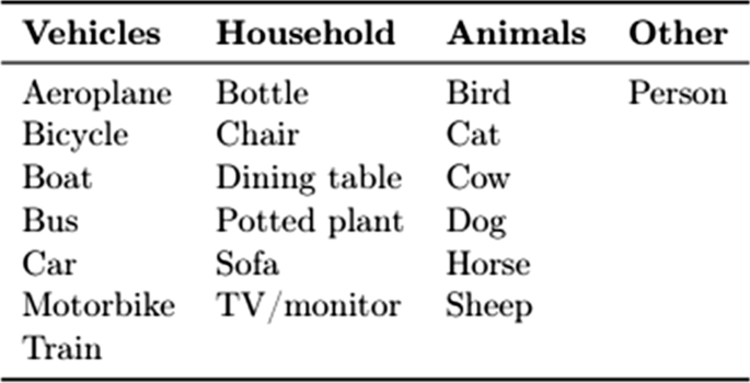
The classes of objects considered in the challenge [43]
Statistics of the VOC2012 datasets [43]
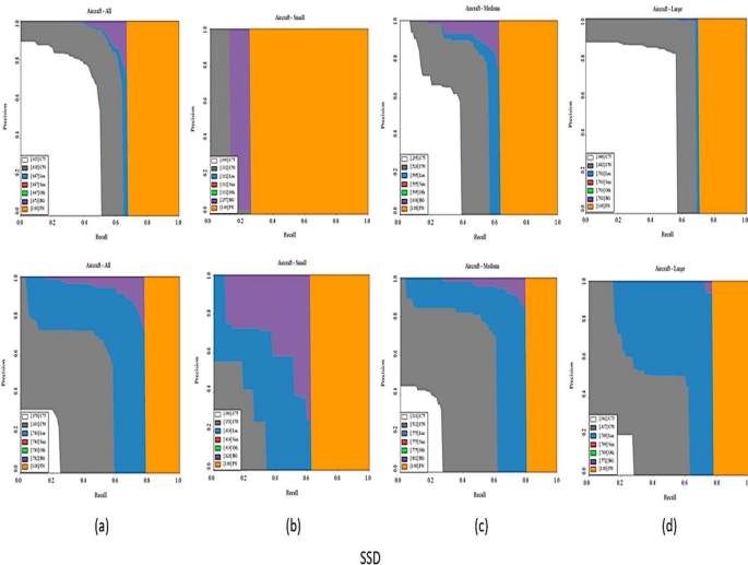
Graph for SSD [26]
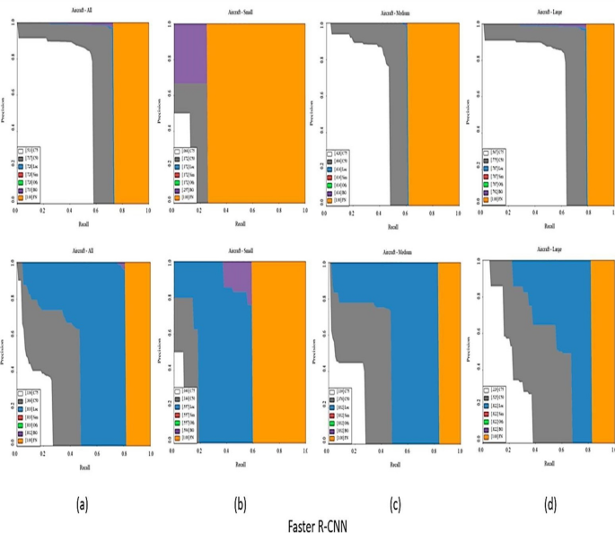
Graph for faster RCNN [26]
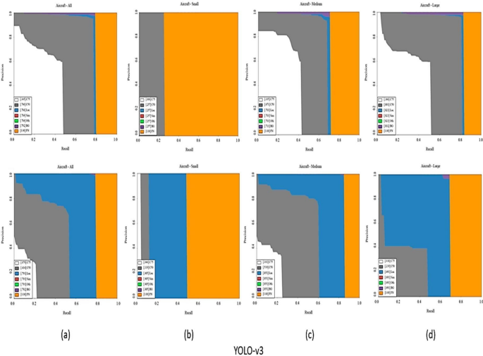
Graph for YOLO [26]
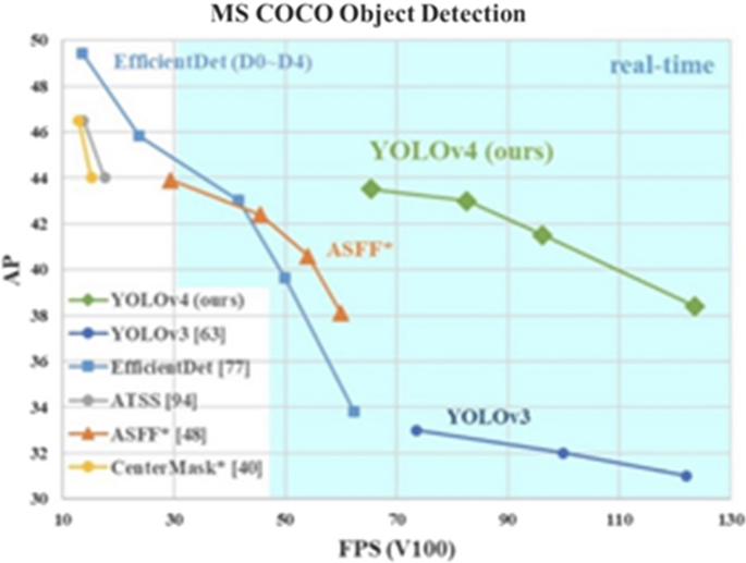
Compared with YOLOv3, the new version of AP (accuracy) and FPS (frame rate per second) are improved by 10% and 12%, respectively [46]
Software
The software configuration put to use is the Google Colab using inbuilt engine called Python 3 Google Compute Engine Backend. It provides a RAM of 12.72 GB of which 3.54 was used at an average. Also, it provides a disk space of 107.77 GB of which 74.41 GB was used which included the training and validation datasets. The hardware accelerator used was the synthetic GPU offered by Google Colab (Tables 1 and 2).
Results and discussions
Two performance metrics are applied to object detecting models for testing. These are ‘Average Precision’ and an F1 score. The predicted bounding boxes are compared with the ground truth bounding boxes by the detector according to IOU (Intersection Over Union). The ‘True Positive’, ‘False Negative’, and ‘False Positive’ are defined and then used for the calculation of precision and recall which in turn are used for calculating the F1 score. The Formulae for these are as follows. [42]
Precision = TP/ (TP +FP’)
Recall = TP/ (TP + FN’)
And using these, F1 score = 2*Precision*Recall/(Precision + Recall)
Apart from these two, the performance of the models is also measured using the following metrics given by the COCO metrics API. [42]
Using all these, the outcomes for all three algorithms were compared in order to compare their performance. The outcomes were as follows:
Results comparison
Discussion
Following were some limitations that were observed in the three models
SSD
When it comes to smaller objects, SSD’s performance is much worse as compared to Faster R-CNN. The main reason for this drawback, is that in SSD, higher resolution layers are responsible for detecting small objects. However, these layers are less useful for classification as they contain lower-level features such as colour patches or edges, thereby reducing the overall performance of SSD [8].
Another limitation of this method which can be inferred from the complexity of SSD’s data augmentation, is that SSD requires a large amount of data for training purposes. This can be quite expensive and time-consuming depending on the application [8]
Faster R-CNN
Accuracy of this algorithm comes at the cost of time complexity. It is significantly slower than the likes of YOLO.
Despite improvements over RCNN and Fast RCNN, it still requires multiple passes over a single image unlike YOLO [3]3
FRCNN has many components—the convolutional network, Regions of Interest (ROI) pooling layer and Region Proposal Network (RPN). Any of these can serve as a bottleneck for the others [3].
YOLO
YOLOv3 was one of the best modifications that had been done to an object detection system since the introduction of Darknet 53. This modified update was received very well among the critics and other industrial professionals. But it had its own shortcomings. Though YOLOv3 is still considered to be a veteran, the complexity analysis showed flaws and lacked optimal solutions to the loss function. It was later rectified in an optimized model of the same and was later used and tested for functionality enhancements [45].
A better version of a given software is the best to analyse the faults in the former. After analysing the paper on YOLOv4 we can see that version 3 used to fail when the image had multiple features to be analysed but they weren’t the highlight of the pic. The lack of accuracy was always an issue when it came to smaller images. It was basically useless to use version 3 to analyse small images because the accuracy was around 16% (proven by our data). Another matter to be looked at is that the use of Darknet 53. YOLOv4 has brought in CSPDarknet-53 which is better than Darknet-53 as it uses only 66% of the number of parameters that version 3 used to use but gives a better result which enhanced speed and accuracy [46].
The precision-recall curves plotted using the COCO metric, API, allowed us to form proper deductions about the efficiency with which these three models perform object detection. Graphs were plotted for each model based on different object sizes.
The area shaded in orange indicates the precision-recall curve without any errors, the area shaded in violet indicates the objects that were falsely detected, the area shaded in blue indicates the localisation errors (Loc). Lastly, the areas under the precision-recall curve that are white indicates an IoU value greater than 0.75 and area shaded in grey indicates an IoU value greater than 0.5.
From the graphs of the three models, it is evident that both region-based detectors like F R-CNN and SSD both have low accuracy due to their relatively larger violet areas. However, amongst themselves, F R-CNN is more accurate than SSD while SSD is more efficient for real-time processing applications due to its higher mAP values. YOLO is clearly the most efficient of the all evident from its almost non-existent violet regions.
Conclusion
This review article compared the latest and most advanced CNN-based object detection algorithms. Without object detection, it would be impossible to analyse the hundreds of thousands of images that are uploaded to the internet every day [42]. Technologies like self-driving vehicles that depend on real-time analysis are also impossible to realize without object detection. All the networks were trained with the open-source COCO dataset by Microsoft, to ensure a homogeneous baseline. It was found that Yolo-v3 is the fastest with SSD following closely and Faster RCNN coming in the last place. However, it can be said that the use case influences which algorithm is picked; if you are dealing with a relatively small dataset and don’t need real-time results, it is best to go with Faster RCNN. Yolo-v3 is the one to pick if you need to analyse a live video feed. Meanwhile, SSD provides a good balance between speed and accuracy. Additionally, Yolo-v3 is the most recently released of the three and is actively being contributed to by the vast open-source community. Hence, in conclusion, out of the three Object Detection Convolutional Neural Networks analysed, Yolo-v3 shows the best overall performance. This result is similar to what some of the previous reports have obtained.
A great deal of work can still be done in the future in this field. Every year, either new algorithms or updates to existing ones are published. Also, each field—aviation, autonomous vehicles (aerial and terrestrial), industrial machinery, etc. are suited to different algorithms.
These subjects can be explored in detail in the future.
Availability of data and materials
Coco dataset used in the paper is available from the website https://cocodataset.org/#explore.
Abbreviations
- FRCNN:
-
Faster Region based Convolutional Neural Network
- SSD:
-
Single Shot Detector
- YOLOv3:
-
You Look Only Once version 3
- COCO:
-
Common Objects in Context
- VGG16:
-
Visual Geometry Group 16
References
Pathak AR, Pandey M, Rautaray S. Application of deep learning for object detection. Procedia Comput Sci. 2018;132:1706–17.
Palop JJ, Mucke L, Roberson ED. Quantifying biomarkers of cognitive dysfunction and neuronal network hyperexcitability in mouse models of Alzheimer’s disease: depletion of calcium-dependent proteins and inhibitory hippocampal remodeling. In: Alzheimer's Disease and Frontotemporal Dementia. Humana Press, Totowa, NJ; 2010, p. 245–262.
Ren S, He K, Girshick R, Sun J. Faster r-cnn: Towards real-time object detection with region proposal networks. IEEE Trans Pattern Anal Mach Intell. 2016;39(6):1137–49.
Ding S, Zhao K. Research on daily objects detection based on deep neural network. IOP Conf Ser Mater Sci Eng. 2018;322(6):062024.
Kim C, Lee J, Han T, Kim YM. A hybrid framework combining background subtraction and deep neural networks for rapid person detection. J Big Data. 2018;5(1):22.
Redmon J, Divvala S, Girshick R, Farhadi A. You only look once: Unified, real-time object detection. In: Proceedings of the IEEE conference on computer vision and pattern recognition; 2016, pp. 779–788.
Ahmad T, Ma Y, Yahya M, Ahmad B, Nazir S. Object detection through modified YOLO neural network. Scientific Programming, 2020.
Liu W, Anguelov D, Erhan D, Szegedy C, Reed S, Fu CY, Berg AC. Ssd: single shot multibox detector. In: European conference on computer vision. Cham: Springer; 2016, p. 21–37.
Womg A, Shafiee MJ, Li F, Chwyl B. Tiny SSD: a tiny singleshot detection deep convolutional neural network for real-time embedded object detection. In: 2018 15th conference on computer and robot vision (CRV). IEEE; 2018, p. 95101
Chen W, Huang H, Peng S, Zhou C, Zhang C. YOLO-face: a real-time face detector. The Visual Computer 2020:1–9.
Fan D, Liu D, Chi W, Liu X, Li Y. Improved SSD-based multi-scale pedestrian detection algorithm. In: Advances in 3D image and graphics representation, analysis, computing and information technology. Springer, Singapore; 2020, p. 109–118.
Mittal P, Sharma A, Singh R. Deep learning-based object detection in low-altitude UAV datasets: a survey. Image and Vision Computing 2020:104046.
Kaplan A, Haenlein M. Siri, Siri, in my hand: Who’s the fairest in the land? On the interpretations, illustrations, and implications of artificial intelligence. Bus Horiz. 2019;62(1):15–25.
Mitchell T. Machine learning. New York: McGraw Hill; 1997.
Schulz H, Behnke S. Deep learning. KI-Künstliche Intelligenz. 2012;26(4):357–63.
Khan A, Sohail A, Zahoora U, Qureshi AS. A survey of the recent architectures of deep convolutional neural networks. Artif Intell Rev. 2020;53(8):5455–516.
Hubel DH, Wiesel TN. Receptive fields, binocular interaction and functional architecture in the cat’s visual cortex. J Physiol. 1962;160(1):106–54.
LeCun Y, Bottou L, Bengio Y, Haffner P. Gradient-based learning applied to document recognition. Proc IEEE. 1998;86(11):2278–324.
Ranzato MA, Huang FJ, Boureau YL, LeCun Y. Unsupervised learning of invariant feature hierarchies with applications to object recognition. In: 2007 IEEE conference on computer vision and pattern recognition. IEEE; 2007, p. 1–8.
Nickolls J, Buck I, Garland M, Skadron K. Scalable parallel programming with cuda: Is cuda the parallel programming model that application developers have been waiting for? Queue. 2008;6(2):40–53.
Krizhevsky A, Sutskever I, Hinton GE. Imagenet classification with deep convolutional neural networks. Adv Neural Inf Process Syst. 2012;25:1097–105.
Simonyan K, Zisserman A. Very deep convolutional networks for large-scale image recognition. arXiv preprint arXiv:1409.1556; 2014.
Girshick R, Donahue J, Darrell T, Malik J. Rich feature hierarchies for accurate object detection and semantic segmentation. In: Proceedings of the IEEE conference on computer vision and pattern recognition; 2014, p. 580–7.
Girshick R. Fast r-cnn. In: Proceedings of the IEEE international conference on computer vision; 2015, p. 1440–8.
Redmon J, Farhadi A. Yolov3: an incremental improvement. arXiv preprint arXiv:1804.02767; 2018.
Alganci U, Soydas M, Sertel E. Comparative research on deep learning approaches for airplane detection from very high-resolution satellite images. Remote Sensing. 2020;12(3):458.
Zhao ZQ, Zheng P, Xu ST, Wu X. Object detection with deep learning: a review. IEEE Trans Neural Netw Learn Syst. 2019;30(11):32123232.
Reza Z. N. (2019). Real-time automated weld quality analysis from ultrasonic B-scan using deep learning (Doctoral dissertation, University of Windsor (Canada)).
Shen X, Wu Y. A unified approach to salient object detection via low rank matrix recovery. In: 2012 IEEE conference on computer vision and pattern recognition. IEEE; 2012, p. 853–60.
Zeiler MD, Fergus R. Visualizing and understanding convolutional networks. In: European conference on computer vision. Cham: Springer, 2014, p. 818–33.
Uijlings JR, Van De Sande KE, Gevers T, Smeulders AW. Selective search for object recognition. Int J Comput Vision. 2013;104(2):154–71. https://doi.org/10.1007/s11263-013-0620-5.
Wu J. Complexity and accuracy analysis of common artificial neural networks on pedestrian detection. In MATEC Web of Conferences, Vol. 232. EDP Science; 2018, p. 01003.
He K, Zhang X, Ren S, Sun J. Identity mappings in deep residual networks. In: European conference on computer vision. Cham: Springer; 2016, p. 630–45.
Xu D, Wu Y. Improved YOLO-V3 with DenseNet for multi-scale remote sensing target detection. Sensors. 2020;20(15):4276.
Butt UA, Mehmood M, Shah SBH, Amin R, Shaukat MW, Raza SM, Piran M. A review of machine learning algorithms for cloud computing security. Electronics. 2020;9(9):1379.
Ketkar N, Santana E. Deep learning with Python, vol. 1. Berkeley: Apress; 2017.
Jiang R, Lin Q, Qu S. Let blind people see: real-time visual recognition with results converted to 3D audio. Report No. 218, Stanford University, Stanford, USA; 2016.
Szegedy C, Liu W, Jia Y, Sermanet P, Reed S, Anguelov D, Rabinovich A. Going deeper with convolutions. In: Proceedings of the IEEE conference on computer vision and pattern recognition; 2015, p. 1–9.
Zhao L, Li S. Object detection algorithm based on improved YOLOv3. Electronics. 2020;9(3):537.
Syed NR. A PyTorch implementation of YOLOv3 for real time object detection (Part 1). [Internet] [Updated Jun 30 2020]. https://nrsyed.com/2020/04/28/a-pytorch-implementation-of-yolov3-for-real-time-object-detection-part-1/. Accessed 02 Feb 2021.
Ethan Yanjia Li. Dive really deep into YOLOv3: a beginner’s guide. [Internet][Posted on December 30 2019] Available at https://yanjia.li/dive-really-deep-into-yolo-v3-a-beginners-guide/. Accessed 31 Jan 2021.
COCO. [Internet]. https://cocodataset.org/#explore. Accessed 28 Oct 2020.
Everingham M, Eslami SA, Van Gool L, Williams CK, Winn J, Zisserman A. The pascal visual object classes challenge: a retrospective. Int J Comput Vision. 2015;111(1):98–136.
Everingham M, Van Gool L, Williams CK, Winn J, Zisserman A. The pascal visual object classes (voc) challenge. Int J Comput Vision. 2010;88(2):303–38.
Huang YQ, Zheng JC, Sun SD, Yang CF, Liu J. Optimized YOLOv3 algorithm and its application in traffic flow detections. Appl Sci. 2020;10(9):3079.
Bochkovskiy A, Wang CY, Liao HYM. Yolov4: optimal speed and accuracy of object detection. arXiv preprint arXiv:2004.10934, 2020.
Acknowledgements
Not applicable.
Funding
Not applicable.
Author information
Authors and Affiliations
Contributions
SS: Research and Implementation of YOLO Algorithm. Comparative Analysis. AVD: Research and Implementation of Faster RCNN Algorithm. Comparative Analysis. CA: Research and Implementation on Faster RCNN Algorithm. Comparative Analysis. IN: Research and Implementation of SSD Algorithm. Comparative Analysis. VK: Research and Implementation on SSD Algorithm. Comparative Analysis. VP: Verification of results obtained through implementations. Approval of final manuscript.
Corresponding author
Ethics declarations
Ethics approval and consent to participate
Not applicable.
Consent for publication
Not applicable.
Competing interests
The authors declare that they have no competing interests.
Additional information
Publisher's Note
Springer Nature remains neutral with regard to jurisdictional claims in published maps and institutional affiliations.
Rights and permissions
Open Access This article is licensed under a Creative Commons Attribution 4.0 International License, which permits use, sharing, adaptation, distribution and reproduction in any medium or format, as long as you give appropriate credit to the original author(s) and the source, provide a link to the Creative Commons licence, and indicate if changes were made. The images or other third party material in this article are included in the article's Creative Commons licence, unless indicated otherwise in a credit line to the material. If material is not included in the article's Creative Commons licence and your intended use is not permitted by statutory regulation or exceeds the permitted use, you will need to obtain permission directly from the copyright holder. To view a copy of this licence, visit http://creativecommons.org/licenses/by/4.0/.
About this article
Cite this article
Srivastava, S., Divekar, A.V., Anilkumar, C. et al. Comparative analysis of deep learning image detection algorithms. J Big Data 8, 66 (2021). https://doi.org/10.1186/s40537-021-00434-w
Received:
Accepted:
Published:
DOI: https://doi.org/10.1186/s40537-021-00434-w
