Experimenting sensitivity-based anonymization framework in apache spark

Abstract

One of the biggest concerns of big data and analytics is privacy. We believe the forthcoming frameworks and theories will establish several solutions for the privacy protection. One of the known solutions is the k-anonymity that was introduced for traditional data. Recently, two major frameworks leveraged big data processing and applications; these are MapReduce and Spark. Spark data processing has been attracting more attention due to its crucial impacts on a wide range of big data applications. One of the predominant big data applications is data analytics and anonymization. We previously proposed an anonymization method for implementing k-anonymity in MapReduce processing framework. In this paper, we investigate Spark performance in processing data anonymization. Spark is a fast processing framework that was implemented in several applications such as: SQL, multimedia, and data stream. Our focus is the SQL Spark, which is adequate for big data anonymization. Since Spark operates in-memory, we need to observe its limitations, speed, and fault tolerance on data size increase, and to compare MapReduce to Spark in processing anonymity. Spark introduces an abstraction called resilient distributed datasets, which reads and serializes a collection of objects partitioned across a set of machines. Developers claim that Spark can outperform MapReduce by 10 times in iterative machine learning jobs. Our experiments in this paper compare between MapReduce and Spark. The overall results show a better performance for Spark’s processing time in anonymity operations. However, in some limited cases, we prefer to implement the old MapReduce framework, when the cluster resources are limited and the network is non-congested.

Introduction

Big data evolution has formed new software tools and techniques to accelerate the processing speed, and increase the scalability. The new tools targeted many big data applications such as data analytics. The analytics has manifested some security concerns, as a reason for big data publicity prominence. In general, big data is more beneficial when it is shared among multiple entities. This means many organizations from different fields need to access this data for multiple purposes [1]. They all analyze, mine, and output statistical results. However, exposing any private data to public view carries a high-security risk. Personal re-identification is the focus of researchers since decades. In data analytics, adversaries can easily re-identify and violate some private information. The information may contain sensitive information about patients, bank agents, census, or any other private information [2].

The previously mentioned methods focused on developing algorithms to determine the best cut of the taxonomy tree, the optimal values of k, and/or the best option of anonymization technique either by Top–Down Specialization (TDS) or by Bottom–Up Generalization (BUG). Implementing these algorithms may require high computation costs of continuous iterations with conditional statements, which means multiple times of heavy scan for the whole data records. However, these algorithms have ignored two main facts about big data processing; the first fact is that the key success factors of parallel processing is a proper parallelization algorithm [3]. This can be achieved by reducing the iteration to the minimal possible level. This is essential to avoid multiple scans for large data records. The major concern is not only the time consumption, but the unexpected failure that arbitrarily occurs during big data processing. The second fact is the changes that occur in data growth. With the increased number of data records, data gain more similarity in attribute’s values. This is apparent in our life activities. For instance, if we sit in a data hall with 100 people, and the probability of finding a person’s age = 33 is 1%, then the probability of finding the same age may go up to 10%, if the data hall contains 1000 people. This is because people’s age range is between [0 and 100], so more people will increase the value equivalency.

The previously mentioned facts are essential to understanding big data nature and specifications. Applying heavy computation to a certain group of data records to find out the best anonymization cut, or even to decide which attribute that we need to anonymize, is inadequate. In big data, applying such techniques may not affect the final results of statistical output. We even may ignore the small statistical value of small decimal results. The statistical results follow the principle of estimation prospect, which gives data miners a flexibility of approximating and rounding some numbers [4]. Therefore, pre-calculating the k value, and pre-determining the attributes needed to be anonymized is an advantage. Generally, this non-accuracy will not dramatically affect the data analytics results.

We introduce a novel anonymization method using Bottom–Up Generalization in k-anonymity that can address the previous two facts about big data. The method utilizes Multi-Dimensional Sensitivity-Based Anonymization for big data (MDSBA). The main aim of our method is to improve the anonymization performance and to increase the usefulness of anonymized data. MDSBA is not only an anonymization algorithm or technique, but it provides a fine-grained access control for multi-level of user’s permissions. MDSBA is further explained in “Background” section.

In this paper, we experiment our MDSBA approach in two different frameworks for big data. We apply k-anonymity in MapReduce framework and compare it with Spark. Spark is an in-memory cluster computing framework for processing and analyzing large amounts of data. It exploits the increased size of hardware resources in CPU and RAM. Nowadays, Spark is the most popular processing framework for big data, by providing cost-effective and high scalable processes. MapReduce and Spark are both popular open source cluster computing frameworks. These frameworks are used in big data for large-scale data analytics, by applying parallel distributed processing tasks. Both frameworks provide programming API to users on managing major components of mapping, shuffling, execution, and caching [5].

Our contribution in this paper is correlated to our previous experiments and researches, which are part of the personal de-identification studies. This research is one of a few studies that elaborated k-anonymity in MapReduce ecosystems. Moreover, the paper introduced a novel method in de-identification by implementing MDSBA in Apache Spark. This method proposes a state of the art for k-anonymity in big data. The current k-anonymity methods do not propose real solutions in big data environment. They suffer from lack of efficiency and scalability, and do not provide appropriate solutions for big data over the cloud network such as granular access for data analytics.

To elaborate on these points, the rest of this paper is structured as follows. Four sections are presented in the rest of this paper as follows: “Background”, “Methods/experimental”, “Results and discussion”, and “Conclusion”. In the “Background” section, the paper describes some previously proposed methods in k-anonymity. The section consists of the related previous work, followed by MDSBA structure and core method. The subsection "Spark structure" describes Spark components and structure and sets the scene for the next parts. We then summarize a general comparison of Spark and MapReduce in subsection "MapReduce and Spark". This is followed by reasons and explanations of choosing Spark framework over other available big data frameworks, such as Flink or Storm, in subsection "Choosing Spark". In “Methods/experimental” section, a general introduction for the Results and Discussion’ is presented. In subsection "Implementing MDSBA in Spark", we explain the algorithm that is implemented to anonymize data by MDSBA method. Part of this subsection describes the User-Defined Function (UDF) implemented in the anonymization program. The last subsections explains the method of comparing between MapReduce and Spark. The method includes the setup of the university lab and a description of the dataset being used in the experiments. The “Results and discussion” section sets an experimental comparison between Hadoop ecosystems, presented by Pig script, and Spark, presented by Scala script. In “Conclusion” section, we summarize the experiments results and findings.

Background

Related work

The K-anonymity method was initially proposed by Sweeney. K-anonymity suggests a data generalization and suppression for Quasy-Identifier (Q-ID) [6]. The Q-ID involves finding a group of attributes that can identify other tuples in the database. These identifiers may not gain 100% of data, but the risk of predicting some data remains high. The original k-anonymity method defines minimum generalization and maximum generalization. It guarantees privacy when releasing any record by attaching each record to at least k individuals, and this is correct even if the released records are connected to external information. Any table is called k-anonymous if one tuple has Q-ID values, and at least k − 1 equivalent records have Q-ID values. This means that the equivalence group size on Q-ID is at least k [7].

Anonymization methods, based on k-Anonymity, have been widely employed to prevent data re-identification [7]. Anonymization methods fall into two broad categories. The first category constitutes of techniques that generalize data from the bottom of the taxonomy tree towards its top and are referred to as the Bottom–Up Generalization (BUG) [8]. The second one is based on walking through the taxonomy tree from the top towards the bottom, known as the Top–Down Specialization (TDS) [9]. TDS and BUG methods were mainly developed for traditional data. Therefore, researchers upgraded the old methods to suit the new operations of big data. The operations should consider the parallel and distributed processing steps. Various methods of anonymization were specifically designed for parallel distributed processing. However, most resolutions fall short of a proper parallelization capability. The reason for this is further explained in this review.

The previous BUG and TDS methods have also been implemented in big data anonymization. A few amendments were applied to suit the big data frameworks regarding parallelization and distribution. The core concept of k-anonymity is similar to the previously mentioned methods. Similar techniques and algorithms are applied in both cases of TDS and BUG. Let us study some of these anonymization methods to compare the previously mentioned methods in traditional data and big data.

BUG was proposed recently for anonymization using MapReduce. Some of BUG algorithms are Parallel BUG [10], and Hybrid BUG. Most BUG methods follow a similar algorithm by implementing the BUG driver to leverage information gain and security trade-off. The search metric computes the Information Loss per Privacy Gain (ILPG). These equations measure the entropy and scores of each attribute. The algorithm generates a random number (ran). This number presents the number of random partition for the dataset ($DS_{ran}$). Each sub-dataset is emitted to the MapReduce BUG (MRBUG) driver for intermediate generalization. This generalization scans data, finds the equivalent records < k and merges Q-IDs up to Anonymization Level 1 or 2—that is, AL1 or AL2. This intermediate generalization is essential to reduce the final anonymization computation. Finally, the datasets are scanned again and the search metric computes ILPG again. For each sub-dataset, if < k, then the best generalization level is found and set to inactive. The process keeps iterating and moving up the taxonomy tree until k-anonymity is satisfied. As explained, the MRBUG driver operates twice—in intermediate and final. It first merges anonymization and then applies generalization. This algorithm is found in [10,11,12,13].

Pandilakshmi et al. [12] proposed advanced BUG. Advanced BUG consists of the following steps: split data into smaller partitions, run the MRBUG driver on a partitioned dataset, combine the anonymization levels of the partitioned dataset and apply generalization to the original dataset [14]. Other anonymization methods use a hybrid combination of BUG and TDS to anonymise data. A threshold value of k is determined by several algorithms to distinguish BUG from TDS use. The proposed methods consider that BUG is more suitable for small k values, while TDS is more suitable for larger k values [15]. Some hybrid methods were recently proposed for big data by Zhang et al. and Irudayasamy et al. [10, 11, 16].

Since the evolution of MapReduce and parallel processing, Roy et al. presented a data privacy model named Airavat [17]. This system was developed after investigating MapReduce and differential privacy. This approach has encouraged researchers to redesign the available anonymization methods for MapReduce computability. The TDS methods for big data were derived from the TDS proposed for traditional data. Minor corrections have been contributed to the early versions of the MapReduce framework. One of the predominant methods is known as two-phase TDS.

Two-phase TDS depicts the two phases of map and reduce. The concept is very similar to the previously explained TDS, which depends on generalizing all Q-ID attributes, and calculating the entropy and score for each Q-ID. The highest Q-ID score will be specialized. This operation is iterated to find the best cut in the tree or in the interval. In the first phase, dataset D is split into small chunks of data, Di. Di denotes any block of data, where $1 \le i \le p$. The value $p$ denotes the number of blocks. An operation known as MapReduce TDS (MRTDS) scans each data block in a subroutine in parallel to make full use of the job-level parallelization of MapReduce. The MRTDS driver is an intermediate anonymization level that specializes data without violating k-anonymity. The MRTDS driver is applied once in each phase. In the first phase, the driver provides some sub-datasets of a $k^{I}$ value, where $k^{I} > k$. The term $k^{I}$ denotes the intermediate anonymity parameter, which is usually given by anonymization experts. Formally, the MRTDS operates multi-tasks on each data block for initial specialization by $MRTDS\left( {D_{i} ,k^{I} ,AL^{0} } \right) \to AL_{i}^{ |}$. The anonymization level $AL^{0}$ presents the top generalization level of the taxonomy tree, which is usually given by (any). Specializing Q-ID attributes is applied as per the highest score attribute. Another program is known as Information Gain per Privacy Loss (IGPL). The IGPL calculates the highest score for each specialized Q-ID attribute. This technique is popular in most anonymization operations and algorithms.

After completing the intermediate anonymization, all (AL) values are aggregated and the next phase is initiated. The second phase operates MRTDS again to produce the best cut specialization. The algorithm is similar to the first phase algorithm. The second phase receives data from the intermediate output as per the key-value of (key, list(count)). This phase updates the IGPL results that were initiated in the first phase. Initially, the first phase lists all best specializations for each data block. In the second phase, the specialization is validated or updated with a new specialization value. The validation is accomplished by attaining two conditions. First, the parent value of specialization should not be a root—that is, it should not be (any). Second, the anonymity should be $A_{c} \left( {spec} \right) > k$. Several iterations can determine the best specialization cut for the chosen Q-ID. The IGPL updates the specialization list as per the information gain calculation, and the final list of specialization is updated and emitted, so the data records are masked with this list [18].

Multi-dimensional sensitivity-based anonymization

We introduce a novel anonymization method using BUG in k-anonymity that can cope with the big data frameworks. The method does not only parallelize data for big data frameworks, but also reduces the computation overhead of data iteration, by providing pre-calculated k-anonymity parameters and pre-determined attributes for anonymization. The MDSBA also supports the access control based on anonymization. This imposes a granular anonymization based on user’s access level. MDSBA mimics role-based access control by providing a granular security access for multi-user levels. The granularity is gained by implementing three different techniques; the probability value of Q-ID attributes, the ownership level $\bar{k}$, and the grouping method of Quasi Identifiers (Q-ID). The Q-ID probability is an essential part on applying masking of taxonomy tree, interval or suppression [19]. The probability value is derived from the taxonomy tree concept. The taxonomy tree T is propagated from the parent node w to the number of child leaves ∑ν, so each parent node’s probability is $P\left( w \right) = \frac{1}{\sum v }$. The intervals, also presented by probability values. The ownership level ($\bar{k}$) is a small value of k-anonymity. It is a number given to each user on accessing data for analytics. This number indicates the minimum number of equivalent Q-ID records, so $\bar{k}$ is usually smaller than or equal k. The larger value of $\bar{k}$ implies a higher level of anonymization.

In order to parallelize massive size of data, and to support the anonymization granularity, we logically divide the Quasi Identifiers (Q-ID) into small groups of two to four Q-IDs, with one class attribute. Each Q-ID group, G(QID), is mapped to a business role and given a fixed value of k. In such a way, users are given authorization rights to access some Q-ID groups as per their given business role. Mapping Business roles and groups were further discussed in this paper [20]. Let us study the following example, if two users, user1 and user2, have requested to access the following Q-ID groups; G(QID)1 = {age, job, suburb, salary(class)}, and the other Q-ID group, G(QID)2 = {admission_date, cancer_found(yes/No), diagnosis(class)}. G(QID)1 is mapped to Finance Manager, and given a value of k = 30, and G(QID)2 is mapped to Doctor and given a value of k = 20. Suppose that user1 was given a Doctor role, and user2 was given a Finance Manager role. Each one of these users will be given a value of $\bar{k}$ to represent the ownership level, which provides an access granularity. The value of $\bar{k}$ is assigned to users based on the service level of agreement, the trust level, and other considerations. More details regarding $\bar{k}$ assignments are available in a previous paper as mentioned here [21]. The value of $\bar{k}$ is an integer number with a pre-condition of 2 ≤ $\bar{k}$ ≤ k. In our example, if the organization of user1 and user2 is belong to one of the data owner’s partners, then users will be given high access privileges, and the value of $\bar{k}$ will be low. Users will be possibly given, user1 → $\bar{k} = 10$, and user2 → $\bar{k} = 5$.

Referring to the previous example, MDSBA pre-calculates the anonymization masking level based on the given value of $\bar{k}$. Mathematical equations are used to calculate the sensitivity level ψ. The equations provide the minimum level of the taxonomy tree on anonymizing Q-ID attributes. The equation is further described in here [22]. It also provides the minimum interval length on anonymizing Q-ID attributes. These pre-calculated data save the time of expensive computation to find the best cut and the best interval. The pre-calculated values are essential in big data to reduce the processing cost. The current anonymization methods spend considerable time calculating the most accurate Q-ID for anonymization. MDSBA neglects this kind of accuracy; thus, the pre-calculation of parameters is straightforward and does not require a high amount of processing. It is apparent that reducing the computation cost may negatively affect the information gain percentage. MDSBA was not proposed for traditional data size; instead, it was developed to leverage large data size, where small changes in accuracy may not affect the final statistical results. In addition, Pre-calculating the value of k is accomplished by reasonably accurate mathematical equations such as linear regression [21].

Moreover, every Q-ID Group is anonymized in a separate task. In each Q-ID group, the anonymization algorithm is given the direction of the grouping sequence depending on the probability value of each Q-ID. In the previous example, the anonymization algorithm will first group the whole three Q-ID attributes in G(QID)1 to filter out the fully-equivalent records. The next stage, the anonymization algorithm will group the highest two Q-ID probabilities. The Q-ID probability is pre-calculated as per the Q-ID values, for instance the probability P(age) = 1/100, P(job) = 1/200, and P(suburb) = 1/400. It is obvious that the highest two Q-ID probabilities are P(age) and P(job), while P(suburb) is the lowest. Hence, the grouped Q-IDs will be ‘age’ and ‘job’ in the second stage, because they have the highest probability values. In the final stage, the highest Q-ID probability will be grouped. In our example, P(age) = 0.1 is the highest probability value, thus, it will be grouped. On the other hand, suburb will be anonymized in the second stage, while job and suburb will be anonymized in the final stage. The pre-chosen anonymization masks depend on the data type of each attribute. For instance, the masking methods of the previous example are intervals for age, and taxonomy trees for suburb and job. As explained, it is clear that anonymization parameters are pre-calculated and determined prior the anonymization process kickoff. In big data, this is essential to reduce the number of records scanning on each round.

Spark structure

Spark operations are different from the traditional MapReduce. Spark architecture is implemented to increase process performance by using the maximum capabilities of the available resources. For this reason, multiple jobs can run in parallel by implementing applications, executors and active drivers. The traditional MapReduce splits each job into many tasks, and each task is undertaken by a single process within each container, so the process terminates when the task is completed. Every node consists of one JVM core, unlike with Spark, where each worker node may consist of many cores, and each core operates in one JVM, as shown in Fig. 1. The node may have many cores, depending on the node capacity. Each core comprises one executor process that can run multiple tasks, and remains for the entirety of the Spark life. This structure accelerates the initiation of the process and tasks. In addition, Spark consists of a process, known as an active driver. This driver is used to manage the job flow and schedule tasks, and is located on the master node. It interactively communicates with the executor of each node. If Spark was deployed on top of YARN, the Spark driver can run over the cluster [23].

Fig. 1

Spark structure and job distribution: This Figure shows one worker with multiple executers. It shows the NameNode and jobs dividing between executers. Each executer contains several JVM cores, which utilizes the memory use

One of the negative aspects of Spark is the programming difficulties that programmers may face. Spark operates in RAM, and programming with large data may cause Spark to run out of heap memory because of the unnecessary RDD data collection caused by the programmer algorithm. Programmers should have previous knowledge about Spark core structure and jobs, such as partitions, nodes, serialization, JVM, executors, memory and disk, shuffles, compressed files and columnar formats (parquet). They may need to try various algorithms to deduce the most efficient one. This frustrating and time-consuming code may cause bugs during the program execution as soon as the data exceed the maximum limit of resources. Usually, cached data that do not fit in the memory are either spilled to the disk or recomputed when needed, as determined by the RDD’s storage level. However, this does not prevent data growth bugs and overflow [24].

Anonymity in data analytics is an example of complex analytics, where anonymization operations scan the data records many times during the filtration, aggregation and masking operations. The anonymization process latency is considerably high; therefore, batch processing tools are more efficient to deal with a large data size and long latency. Big data tools were developed to accommodate both data batches and streams. The first generations of MapReduce frameworks, such as Hadoop, were unable to process the data stream. The next generation was developed based on Lambda architecture, which was designed to handle both batch and stream processing methods. The Spark framework structure attempts to trade-off between latency, throughput and fault-tolerance. Most of the real-time frameworks follow a similar structure of storing temporary data frames and tables in the memory, so most of the operations are completed without performing I/O operation with disks, thereby decreasing latency [2].

MapReduce and Spark

Both the Spark and MapReduce frameworks are very similar in some core features. Spark runs on Hadoop, on Mesos or standalone; hence, it is not possible to categorize Spark as a non-MapReduce framework. The MapReduce core structure consists of YARN and HDFS, and these two Hadoop native processes are used intensively in Spark. They provide reliability, performance and scalability for Spark. It is worth mentioning that two notable differences between MapReduce and Spark in processing MDSBA.

• 1. The first factor is that MapReduce wastes considerable time on I/O transmission between memory and disks. The inefficiency of read/write from the disk and the high latency in each operation are the major inhibitors in MapReduce. In contrast, Spark operations are executed over a built-in memory, without a need for read/write on disks [25]. Figure 2 illustrates a comparison of Hadoop and Spark. Spark’s in-memory cluster computing capabilities are high, which boosts performance, even with the large data magnitude. The time difference between reading data from the disk or from the memory is significant. A larger data size shows higher latency than a smaller data size when reading from disks. In addition, Spark implements a caching technique to store data in the memory to minimize the disk I/O.

  Fig. 2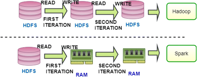

  

  Comparison between Hadoop and Spark in dealing with memory and disks: Hadoop is slower than Spark because it processes each task on two stages, map and reduce. Every two stages must output data to the disk. On the other hand, Spark operates in-memory, therefore, it is faster

• 2. The second factor that enables Spark to operate more rapidly than Hadoop is the advanced job execution engine. Both Spark and MapReduce convert a job into a DAG of stages. The DAG theory is an old theory that represents any graph with a collection of vertices connected by edges [26]. Graph theory was developed and implemented in many fields, such as computer science and medical science. In Hadoop and Spark, graph theory is used for scheduling tasks. Each job is presented by a direct graph, which is a set of vertices connected by directed edges. Each vertex in the graph represents one processor, and each edge represents a communication link. The difference between Spark DAG and Hadoop DAG is the communication link. In Hadoop, each processor reads all incoming messages from the in-edge (disk), performs some computation, and writes messages to the out-edge (disk). The in-edge and out-edge are presented by disk I/O, which causes major delays. Hence, two stages can be processed at a time. In other words, there is no way to start at a vertex in a DAG and follow a sequence of directed edges to return to the same vertex [27]. Hadoop creates a DAG with only two predefined stages: map and reduce. Developers are forced to process their commands within one of these two stages. Based on this core structure, complex jobs need to be split into two or more jobs to fulfil the two-stage process. In contrast, Spark can accomplish the job with multiple stages, without splitting the single job into many sub-jobs. This structure optimizes job scheduling and processing. For instance, if the processing algorithm contains read from storage, filter and group, Spark can accomplish this algorithm in one job with three stages of map, shuffle and reduce. In Hadoop, this would be divided into two jobs of (map, shuffle) and (map, reduce) for each job. Data would be read from the disk, filtered and stored back to the disk with the first job. Again, data would be read from the disk, grouped and stored back to the disk.

Choosing Spark

There have been a considerable number of cluster computation engines available in the market during the last decade, including Hadoop, Spark, Flink, Storm, Heron and Samza. Storm is a viable framework in the big data industry, as it presents a real-time processing engine that is able to stream SQL records from HDFS, Kafka, MongoDB and Redis [28]. Storm is a popular framework worldwide, and is implemented in enterprise company networks, such as Yahoo, Twitter, Flipboard and Yelp. It is written in Clojure Language—the Lisp-like functional language. Moreover, the structural design of Storm was built for the data stream, which means that the Storm process is continuous and infinitive. However, Storm was not selected for data anonymization because it does not process batching datasets—it only operates with data streaming—and anonymization methods and operations are only applied to batching data. This is essential for grouping and counting the number of equivalent records and masking the non-equivalent records. These operations cannot induce adequate anonymization results in the data stream; hence, Storm is not preferable in k-anonymity methods [29].

However, some hinders may degrade the efficiency of Spark. As aforementioned, if the data size does not fit the total memory size of the cluster, then Spark uses disks to spill data. This action causes a higher delay on disk I/O, which is a similar delay factor in the Hadoop framework. Therefore, the Spark cluster always needs a large memory size to leverage the best performance. The average amount of processed data should be considered when building the Spark cluster because Spark has the capability of caching RDD in memory. Developers benefit from this feature to avoid disk I/O; however, caching features requires a sufficiently large memory size. For instance, if the Spark cluster is expected to analyze a data size of 3 TB, then Spark uses up to 60% of the total configured executor memory to cache RDDs. If data analyzers decided to cache half of the 3 TB in-memory at once, there should be enough memory space to accommodate this large data size. In this scenario, a Spark cluster with 20 workers and 128 GB memory for each worker is enough to cache 1.5 TB. A rough calculation is $20 \times 128 \times 0.6 = 1536 GB \approx 1.5 TB$. As explained earlier, the Spark cluster infrastructure should consist of powerful servers and fast connectors between workers and storage units. Therefore, VMs connected to storage nodes by iSCSi are not a suitable choice for building a Spark cluster. Spark requires physical or non-virtual servers. In addition, network connections between servers and storages should be through direct access connection, such as SAS or SATA.

Methods/experimental

Spark has many advantages over Hadoop ecosystems. It mitigates latencies and increases performance. For instance, Pig divides jobs into small tasks, and, for each task, Pig reads data from HDFS, and returns data to HDFS once the process is completed. This in/out consumes considerable time, and is unlike Spark, which implements an RDD. RDD is the main distinguishing feature of Spark. RDD divides jobs into many DAG stages, and, for each stage, Spark reprocesses RDD in the memory without referring to the disk. Spark may perform many times faster than MapReduce.

In this chapter, Pig’s and Spark’s performances are evaluated in MDSBA. To conduct a detailed evaluation, Spark’s transformation and functions used in anonymization should be properly defined. All Spark scripts are coded by Scala program. Some functions and transformations operate faster than others. For example, inner join transformation commands may require a high computational cost. MDSBA was proposed for big data processing frameworks. Its core concept is applying optimized anonymization procedures and algorithms by splitting data into small tasks, so they can be parallelized among the cluster nodes.

In big data processing, the reduce phase is expensive because it involves data partitioning, data serialization and de-serialization, data compression and disk I/O. These operations require data transfer over the network to aggregate data over multiple nodes. Leveraging any application’s behavior should consider the size of data transferring between nodes during the reduce phase [30]. In data anonymization, the reduce phase is presented by SQL grouping commands, which causes high shuffling processes. To reduce the groupBy effect in the anonymization application, a filtration command is initiated to split data logically as per nominal values. This type of split reduces the performance degradation caused by the shuffling process. This reduces the amount of shuffling among cluster nodes during the reduce stage.

Implementing MDSBA in Spark

The previous anonymization techniques, such as BUG and TDS, were supposed to work efficiently in parallel distributed processing. Technically, anonymizing data with these algorithms may negatively create data overflow without considering the cluster resources and capabilities. For instance, Fig. 3 illustrates a comparison of the TDS and MDSBA algorithms. In the TDS algorithm, the data flow may negatively affect parallelization. First, grouping all records without filtering data is inefficient. This is experimentally proven in Spark Tuning in MBA Section. Second, most TDS operational steps should be executed in UDF, which degrades the algorithm performance. Spark and Pig are unable to run intensive computations and conditional iterations without UDF. Therefore, UDF is embedded in the script’s codes to execute complicated operations. However, using UDF in most anonymization steps inhibits the performance of Hadoop and Spark. The operations of UDF are executed in a black box, and are not related to Spark or Hadoop frameworks. This is also true in Pig operations. UDF does not use the resources of YARN; instead, it uses the resources of locally installed JVM. Therefore, implementing Spark with such an algorithm is inefficient.

Fig. 3

Comparison between the anonymization algorithms of MDSBA and TDS: MDSBA reduces the dependencies on UDF by reducing the iteration steps. TDS requires many iterations to determine the best cut. This improves the scalability and performance of MDSBA

In MDSBA, UDF was embedded in Spark and Pig scripts, but with a minimal size of data processing. As explained in the next section, the anonymization is applied on fewer attributes at a time. This technique controls and minimizes the size of data flowing to the UDF. The UDF is executed in a local JVM beyond the source manager’s control—a memory pool located outside the Spark JVMs. Therefore, there is a need to reduce the amount of data flowing outside the Spark JVMs [24]. Moreover, the anonymized Q-ID in TDS is volatile. This means that the specialization is applied to different Q-ID attributes in each group of records. The chosen attribute for specialization is the attribute with the highest score value [9]. Calculating the highest attribute score for each group is an expensive computation process. In contrast, in MDSBA, the anonymized Q-ID is predetermined based on the Q-ID probability. This saves a considerable amount of computation time. This solution may not provide the best optimal anonymization for all anonymized groups in the dataset, however, we may sacrifice some information gain to benefit data processing performance.

Figure 3 compares TDS and MDSBA in anonymizing data. The TDS algorithm involves various iterations when calculating the best cut and scores. This type of iteration is inefficient for big data, and even worse when using UDF, where the program executes the UDF code outside the Spark framework. Further, the UDF program needs to iterate a large size of arrays. The UDF executes almost all anonymization processes; thus, there is no real benefit from a parallel distributed system. In contrast, MDSBA implements UDF with a limited data size flow. As shown in Fig. 3, UDF use was reduced to minimal operations. UDF reads only a few data attributes to apply some masking operations. The data size flowing to the UDF is relatively small.

User-defined Functions in MDSBA

MDSBA implements user-defined functions in different locations. This is essential for two main purposes: anonymizing and ungrouping. In anonymizing, three masking types of interval, taxonomy tree and suppression are implemented. These are the only available types of masking for anonymization, and are used by all anonymization methods. Figure 4 shows the algorithm for anonymizing any numerical group. In Scala, the group of objects can be a list or sequence. Minimizing the amount of data when accessing the UDF program is essential to reduce the processing cost and avoid data overflow, as described before.

Fig. 4

Algorithm illustrates the numerical values anonymization: Anonymization can be applied to textual and/or numerical attributes. Here in this algorithm, the numerical anonymization is denoted by an interval that replaces one digital value

It is difficult to predict the failure of non-Spark JVM; therefore, we must keep data flow to the lowest level. For instance, installing JVM in any computer may take up to 25% of the total memory. This size can be reconfigured and enlarged if needed. If the Spark worker memory is large enough to fit the data size, then the external JVM that handles the UDF may be able to handle up to 25% of the data size located in Spark. The size of the UDF heap memory is not the only obstacle—the complex iteration with several IF statements can be another cumbersome factor that degrades the data processes. MDSBA implements a swift algorithm to anonymize data with the minimum number of iterations.

To understand the anonymization algorithm in UDF, let us study the following example; a list of numerical values is given as: a list = {2,3,4,6,12,12,12,18,25,26,26,30}, with $\bar{k}$ = 5. The algorithm anonymizes this list as per ψ value. If ψ = 0.2, then the range = 1/0.2 = 5. The values are arranged in an ascending order. Referring to Fig. 4, the algorithm consists of four sections. The algorithm:

• 1. Initiates some values; length_of_list = 10, minimum = 2 − (2 mod 5) = 0, and medium = 0+5 = 5.

• 2. Starts reading the first object in the list, (2).

• 3. Section 1: IF statement, since the statement is true, then the counter is incremented, rep = 1.

• 4. Section 2: The next IF statement, in Sect. 2, will be skipped, since the object list has not reached the end of it.

• 5. Section 3: In the third IF statement, the algorithm jumps by 4 objects since Remain_to_k_dash = k_dash – rep = 4.

• 6. Section 3: The next number from the list will be 12, and the other parameters will be incremented for the next loop, rep = 1 + 4 + 1 = 6 and object = 5. Also, the medium value has been updated up to 15.

• 7. Section 4: Proceeding to the fourth statement, it is clear that the 6th list number is also 12, so the statement result is false, and the loop continues the second loop with object = 6.

• 8. Section 1: In the second iteration, the first section increments rep up to rep = 7, and reads the value 12, while the sections two, three, and four are skipped.

• 9. Similarly, the third loop increments rep by rep = 8. In the third iteration, the number 18 exceeds the range, and the program skips to the fourth section.

• 10. This is the first time that the fourth statement is true, and the string of all_intervals is generated by an iterated loop of 8 times, so the results will be new_list{[0–15[,[0–15[,[0–15[,[0–15[,[0–15[,[0–15[,[0–15[}.

• 11. In the fourth section the loop generates the new list, and both minimum and maximum are updated by minimum = 15, and maximum = 15 + 5 = 20.

• 12. The next loop updates the medium up to 35, so the final new list is updated by: {[0–15[,[0–15[,[0–15[,[0–15[,[0–15[,[0–15[,[0–15[,[15–35[,[15–35[,[15–35[,[15–35[,[15–35[}.

In a similar algorithm, we can mask data with taxonomy trees as explained in Additional file 1: Appendix S1. The aim of this algorithm is reducing the size of data flowing to the UDF program. This is implemented by masking fewer attributes at a time, then attaching the rest of the data tuples, to the anonymized attributes. We may roughly estimate the size of ten data records by 1 KB, while the size of one attribute of the ten records may not exceed the 20 bytes. This shows that the actual data size flowing to the UDF file may not exceed one-third of the total data size. For this reason, data processing in UDF is not expectedly expensive. Figure 5, shows two algorithms implemented by Pig and Spark. Both are quite similar with minor differences in the data flow between memory and disk. Spark does not need a disk read/write operation. The fully equivalent records (SG) are stored at disks in both programs, as a final output. The semi-equivalent records (SSG) are stored at the disk in Pig program only, as a temporary output. This is the major difference between both programs. Moreover, Pig is not provided with a built-in UDF capability, therefore, an external program, such as Java, should handle the UDF operations. Unlike Spark SQL, which provides a UDF built-in capability by defining a Scala function.

Fig. 5

Anonymization algorithms in Pig and Spark: very similar anonymization algorithms in Pig and Scala. Only minor differences between them

In Spark algorithm, we faced challenges of concatenating the anonymized data with the rest of the attributes in the table. For instance, if a table T contains the following attributes of T = {A,B,C,D}. The anonymization process has finished masking the attribute A, and transformed it to a, that is A → a. Hence, the anonymized attribute {a} needs to be concatenated with the rest of the attributes {B,C,D}, so the new table TA will be TA = {a,B,C,D}. In Scala’s implementation of DataFrames, there is no direct way to zip two DataFrames into one. We can simply work around this limitation by adding indices to each row of the data frames. Then, we inner join DataFrame by these indices. Additional file 2: Appendix S2 presents a full Scala program including UDF.

However, all join operations are known as Cartesian join, which require high number of shuffling between nodes. Therefore, join operation is very expensive, and it is not recommended by Spark developers. Thus, we implemented another way of concatenating without creating an independent DataFrame. To understand the concept of this UDF script, let us give the following example, four Q-ID attributes and one non-Q-ID attribute, Teacher, are presented in Table 1. On grouping the records by three attributes (CLASS, SCHOOL, and LEVEL), TEACHER and MARK collect multiple values in arrays. The script calls the anonymization UDF to anonymize the marks, and concatenates the rest of the attributes in one table. This can be implemented through (withColumn) command. The command syntax is;

$$\begin{aligned} val \, anonymize\_MARK = Grouped\_QID.withColumn\left( {''MARK'', \, AnonUDF\left( {\$ ''MARK''} \right)} \right) \\ .select\left( {''TEACHER'',{''CLASS''},{''SCHOOL''},{''LEVEL''},{''MARK''}} \right). \\ \end{aligned}$$

Table 1 Grouped and anonymized table

Table 1 should be ungrouped for storing or possible further processing. This format of grouped records cannot be easily managed for computation or statistical operations. Ungrouping the grouped data can be accomplished in various ways. The best-found way was creating another UDF that is able to map every sequence to a wrapped array, and rotate the direction of the wrapped array. The aim is converting Tables 1, 2 format. It is clear that the three Q-ID attributes are repeated according to the number of grouped objects in MARK and TEACHER.

Table 2 Illustrates the new state after ungrouping records

The Ungrouping algorithm reads each wrapped array, counts the number of objects, and maps each array with indices. Each wrapped array has a various number of objects; therefore we need to define a function that can update the array size on each wrapped array. Scala defines functions by using (val) or (def) command. In our case, we implement (def), so the command can update the number of array objects, with the following syntax;

This definition is called by the UDF that is able to rotate the direction of the arrays with the following command:

The above UDF ungroups Table 1, and expands the wrapped array to the format of Table 2. In this example, the anonymization UDF outputs the range of marks in one string of values MARK = {[70–80], [70–80], [70–80]}. This string should be converted to a wrapped array before ungrouping it. Converting a string to an array, in Scala, is implemented by the command split(col(MARK)). As noticed, implementing the fastest algorithm relies on several trials of execution before choosing the best method. In general, programming in big data should be carefully considered. This is quite similar to programming multi-task programs on a single computer with multiple processors. The program may not gain any advantage of the multi-core processor without a proper algorithm. For instance, an operation of total = a + b + c + d will run in one core only, while the rest of the cores are in ideal states. The same operation can be completed faster, if the algorithm was amended by tot1 = a + b, tot2 = c + d, and total = tot1 + tot2. Splitting the single operation to three operations of tot1, tot2, and total, enhances the performance and leverages the parallel processing on multiple cores. However, the operation of the total will be completed on one core only. The final result of the total will wait for the parallel operations of tot1 and tot2 to be completed. This operation is known as a sequence operation, which causes the major delay in algorithms [3]. Applying the similar concept to parallel distributed operation mimics the mapping and reducing operations. Reduce is a sequence operation that waits for the mapping completion, and before the shuffling operation start-up. More shuffling leads to a higher operating cost.

The operation of the grouping process is implemented by the built-in transformation command “groupBy”. Alternatively, Scala permits the SQL embedded commands, so the grouping can be implemented in either way of groupBy or Select query. However, groupBy was found to be more efficient in performance wise. Each data tuple or record contains many attributes. As described before, MDSBA creates small Q-ID groups, which includes two to four attributes only. Also, each data record may consist of several G(QID), classes, and non-Quasi attributes. For this reason, we need to groupBy each G(QID) independently, while the rest of the attributes must be aggregated and concatenated with the anonymized G(QID).

Comparison of MapReduce and Spark in processing MDSBA

We conducted experiments to compare between Hadoop ecosystem and Spark in processing MDSBA. The experiments aimed to measure the performance of the old MapReduce framework and the new Spark framework o conducting data anonymity. The performance includes the computation cost, and scalability of each. Since Spark is a distributed in-memory platform, we need to observe Spark’s behavior on data growth. Eventually, Spark was developed for the new powerful servers that are provided with a large size of memory, and a considerable number of CPU cores. Spark is a memory consumer and CPU intensive operator; therefore, each worker should contain a reasonable size of memory and cores. Usually memory size on each worker starts from 16 GB, with two quad-core processors. However, the required size of memory and processor in each worker of the cluster depends on three main factors, these are: the data size, the time required to complete the job, and the number of workers and masters within the cluster.

Experiment setup

We setup our lab at our university, which includes seven virtual machines, with one master and six workers. Each node contains 4 core CPUs of Intel(R) Xeon(R) CPU @ 2.40 GHz, with a physical memory of 8 GB, and the operating system is CentOS 7. Both Spark and Hadoop were setup on the same cluster. Spark 2.1 was setup on Apache Hadoop 2.7. Also, Pig was setup on the NameNode to run the Pig Latin script. We created two different scripts programmed in Pig Latin and Scala. Both scripts must output similar results. To save resources, we executed Pig script first, then Scala script after the completion of Pig script. Adult data [31] was deployed for the experiments. Data was randomly enlarged up to seven different sizes, and these are 2 GB, 5 GB, 7 GB, 10 GB, 15 GB, 20 GB and 30 GB. The size of data sets was chosen related to the limited available resources in our cluster.

The first experiment aimed to compare the processing time between Spark and Pig. Both scripts are designed to read the data files, filter data by class value, group, anonymize and ungroup. The program concept is similar to the algorithm described in Fig. 5. Spark was setup with a total of five workers with 10 cores. The cores are distributed as two cores and 4 GB memory per worker node. The five nodes have 20 GB of memory, with a total of 10 executers.

In the second experiment, one more worker was added to observe Spark’s behavior with the large hardware capacity. The worker node consists of 8 GB memory and two core processors. The previous experiment was conducted by 5 workers and one master, while this experiment was conducted by 6 workers instead. The sixth worker was added to both Pig and Spark clusters. It showed a dramatic increase in Spark performance, which was expected. Figure 7 illustrates the same datasets with the extra worker added to Spark domain and Pig domain. Spark’s processing time showed a slight degradation, when data size exceeded 20 GB. However, the overall performance was better than using five workers only.

Datasets chosen in the experiments

In both experiments we used adult data taken from UCI Machine Learning Repository. The attributes include {AGE, JOB, MARITAL_STATUS, EDU, SOCIAL, RACE, SEX, POSITION, COUNTY, COUNTRY, SALARY}. Attributes are divided into three groups of Q-IDs. The first Q-ID group is G(QID)1 = {AGE, JOB, MARITAL_STATUS,EDU}, where EDU is the class attribute. The second group is G(QID)2 = {SOCIAL, RACE, SEX, POSITION}, where POSITION is the class attribute. And finally, the third group is G(QID)3 = {COUNTY, COUNTRY, SALARY}, where SALARY is the class. For this experiment, we only anonymized group G(QID)1, by grouping Q-IDs for {AGE, JOB, MARITAL_STATUS} in the first stage, then {JOB, MARITAL_STATUS}, in the second stage, and finally {MARITAL_STATUS} only in the third stage. Table 3 shows the dataset attributes and G(QID) groups.

Table 3 Adult dataset and G(QID) groups used in the below experiments

This dataset was chosen based on various considerations. This dataset contains a considerable number of personal attributes. This creates a larger number of Q-IDs, which enables an appropriate aggregation for G(QID) groups. In addition, this dataset has been used in many previous methods and experiments proposed by researchers. Thus, it is worthwhile employing similar datasets for its prominence in data anonymization.

Adult dataset was enlarged up to seven different sizes by using MySql code, which is retrieved and modified from github [32]. This randomly created data mimics the real-world data, by constructing a random sampling. The sampling was implemented by calculating the normal distribution for each Q-ID attribute and a class. The normal distribution was calculated first for the original Adult data. Then data range is assigned for randomness by giving each 100 values a different range. The data ranges were chosen to resemble the normal distribution value for the original data. We followed similar process that was described here [33].

Results and discussion

The results with 5 workers showed a large contrast in processing time between both scripts. Figure 6 showed the processing time for various data sizes. Spark is much faster than Pig in the relatively smaller data size. The relativity is described by comparing the data size with the memory size. In the proper memory size, Spark may reach up to 8× faster than Pig. On data size growth, Spark performance degrades dramatically, so the processing time becomes similar to Pig on data size = 15 GB. More data growth showed better performance for Pig speed in comparison to Spark. Pig does not speed up processes on data growth, but its processing time grows up steadily. On the contrast, the discrete line in Fig. 6 shows an exponential growth for the Spark processing time. SQL Spark consumes more processing time, when the memory is not large enough in comparison with the data size. For instance, when data size = 30 GB, the process time was around 432 min, which is much larger than Pig process time, which was around 350 min.

Fig. 6

Comparison in process-time between Pig and Scala scripts with 5 workers: This is the first experiment where 5 workers and one master are used. The experiment showed a good performance for Spark, when data size is smaller than 15 GB. Pig gains better performance when data size increases dramatically in comparison with the available memory

The results with 6 workers show that Spark performs better than the previous experiment. However, Pig processes showed slight progresses if compared with Spark’s performance. Figure 7 illustrates a high progress and a dramatic decrease of Spark’s processing time, specially when data size exceeded 3 GB. Spark’s process improvement is due to its structure and in-memory operations. MapReduce is prone to network congestion during map or shuffle phases. Spark reduces this negative impact by reducing the data transmission between disks and memory. This feature is essential in the transmission of the network.

Fig. 7

Comparison in process-time between Pig and Scala scripts with 6 workers: This is the second experiment where 6 workers and one master are used. The experiment showed a good performance for Spark, when data size is smaller than 20 GB. Pig gains better performance when data size increases dramatically in comparison with the available memory

The impact of network congestion on Pig performance

Having many trials of experiments with Pig; several tasks took much longer time before throwing errors and terminating the tasks. The engineering structure of MapReduce and Spark is similar to handling the slow tasks. They both implement a speculative execution, which tags any task that takes longer on average than the other tasks from the same job. It clones this slow task and runs it on another node. It will not stop the slow task, but rather run another copy in parallel. This is beneficial in large clusters, whereas small clusters may lose their available resources. However, our university network is not dedicated to MapReduce structure, and suffers from a high network congestion most of the day. In both cases of enabling or disabling Pig’s speculative execution, we experienced an almost similar delay in some tasks. Therefore, we repeated each experiment several times, mainly, in running Pig script. The failure jobs where repeated and excluded from the comparison time. The failure percentage of processing tasks in Pig script was around 4%, which increases with the data growth. Many factors may cause this congestion, such as university virtual environment and connection types between storages and virtual machines. Big data clusters rely on direct access connection (DAC) between nodes and storages. Also, the virtual environment is not recommended for big data structure. Figure 8 shows 319 tasks that were executed by Pig script for various data size. The tasks belong to more than 15 jobs with an average processing time between 10 s to 18 min for the successful tasks. The shown pulses represent the failure tasks after long processing time. The failure tasks increase in parallel with the data size increase.

Fig. 8

A number of 319 Pig script tasks, including repeated tasks: Pig script operates between disks and memory. This creates many interruptions in the busy network. Therefore, the fail percentages in Pig tasks is high. The failure percentage increases parallel with the data size increase

Spark tuning in MDSBA

Tuning Spark is one of the hardest tasks on managing Spark cluster. This requires knowledge, experience, and several experiments. There are no clear instructions on tuning Spark to gain the best performance. Our focus here is on anonymization operations only. Different tasks and applications may require different steps of tuning. In MDSBA, our focus is grouping, ungrouping, and masking data. These three main operations should be organized properly to give the best possible performance. Both ungrouping and masking require UDF programs. In masking, the algorithms should consider the least number of iteration and the smallest size of data. It was explained earlier the importance of reducing the data flowing to the UDF. We experimented several tuning techniques and configurations. Two main tuning concepts are found; these are: filter/group, and cache data.

In SQL grouping, we experimentally found that filtering data, and then grouping it, may reduce the grouping time and enhance the performance. Hence, we need to filter and then group data, rather than jumping to the GROUP command first. It is apparent that grouping data records can replace the command FILTER, so technically, we can group any records without the need for filtering them first. However, to reduce the number of shuffling times and leverages the parallelization, it is better to filter records first. For a better understanding, let us consider a set of passenger’s records as shown in Table 4. If the grouping command included the attributes of; Depart, Arrive, and Flight, then the grouping results can be {ATL, DXB, (Adult, Child), K380}. We also gain similar results if we use filter command first. For instance, if we filter the records with the class value = K380, then data size will be reduced to two records instead of three. Using filter/group commands conclude the same results as using group command alone. However, in performance-wise they are not similar.

Table 4 Passenger’s records example

Figure 9 shows the processing time difference between grouping data after filtration, and grouping data without filtration. Initial data Filtration increases the program performance, and it is beneficial when the attribute values are known, so they can be hardcoded by programmers. In MDSBA, attribute values are pre-added automatically in early preparation stages. MDSBA framework consists of three main services core, initializer, and anonymizer. The Scala script is generated in the Initializer stage by reading dataset parameters and users’ access parameters from two different XML files. User’s XML file is received from the federation service, while dataset XML file is previously uploaded by data owners to the service provider’s servers, parallel with the dataset. MDSBA framework is further explained here [20].

Fig. 9

Process time between filter/group and group only: comparison between using filter and without filter in the algorithm. It was proven that filter can improve the processing performance

The second tuning in Spark is data caching. The percentage of the failure tasks in Spark script was much lower than in Pig script. The percentage was even lower, when using persist command on reading data from disks. As mentioned before, the (persist) command caches the data in memory. Developers may assign the (persist), if data will be read many times for multiple tasks. Our comparison between (persist) and non-persist commands showed a tangible difference in performance between them. We implemented persist command after reading a dataset from the disk. Figure 10 shows a large difference between both cases, where using (persist) reduces the processing time of tasks. The (persist) command is part of Spark tuning to increase the performance efficacy. However, the command is not recommended when the data size is larger than the available memory. If the data size is larger than the memory, then the overloaded memory will be spilled to the disk. Figure 10 illustrates the performance comparison between (persist) and non-persist. The time processing contrast increases with the increase of the data size.

Fig. 10

Performance comparison between caching and non-caching data: also, caching improves the performance. Caching stores big part of the data in-memory, which accelerate the process

These two steps of tuning make a considerable difference in anonymization performance by MDSBA. Before tuning Spark, it is essential to building a robust Spark cluster and nodes. The hardware infrastructure is the major factor for big data operations success and performance. As mentioned earlier, the memory size of each worker, the number of cores, the number of workers, and the network connection between workers and storages, should be large enough to accommodate the massive size of data. Data anonymization and analytics are heavy processes that require a powerful and large cluster specifications.

Conclusion

With the recent big data’s revolutionary growth, various processing frameworks were developed. Some of these frameworks best fit streaming data, while others can be applied to batch data. In this paper, we experimented two of these popular frameworks for our k-anonymity method. Both of Pig and Spark were examined in MDSBA anonymization process. Our aim was paving a reliable ground for MDSBA state-of-the-art anonymization with the most reliable performance. The experiments show few hurdles in each framework. However, Spark is faster in processing MDSBA, and more fault tolerant as an in-memory operations framework. In congested networks, Spark reduces data transmission between memory and disks on serializing data with RDD. Spark can be many times faster than Pig MapReduce in anonymization. To avoid SQL Spark performance degradation, the memory should be larger than the processed data. SQL Spark boosts performance on the large size of memory. Other Spark’s tuning methods that may leverage the anonymization performance are; UDF algorithm, filter/group commands, and caching data in memory. On the other side, MapReduce is an old framework that can perform better when memory resources are quite small. This is conditioned by the network traffic and congestion level. MapReduce may operate on small memory resources, but it requires non-busy network, because it relies on a heavy transmission between memory and disks. In the conclusion, It is recommended to implement MDSBA in Spark framework, however, the cluster infrastructure must be prepared well, by providing enough memory and processor resources for each node.

Our future research will focus on finding a proper method for data stream anonymization. In big data, streaming is an essential type in most data applications. The current anonymization method of MDSBA does not support the data stream anonymization. Most recent big data frameworks provide complete solutions for the data stream. We may need to amend the current MDSBA method to cope with the continuous data streaming.

References

Chen H, Chiang RH, Storey VC. Business intelligence and analytics: From big data to big impact. MIS quarterly. 2012;36:1165–88.
Guller M. Big data analytics with spark. A practitioner’s guide to using spark for large scale data analysis. The expert’s voice in Spark. Berkeley: Apress; 2015. p. 2015. https://doi.org/10.1007/978-1-4842-0964-6.
Kirk DB, Wen-Mei WH. Programming massively parallel processors: a hands-on approach. Morgan kaufmann. 2016
Govindaraju V. Big data analytics. Oxford: Elsevier Science; 2015. p. 2015.
Shi J, Qiu Y, Minhas UF, Jiao L, Wang C, Reinwald B, Özcan F. Clash of the titans: mapreduce vs. spark for large scale data analytics. Proc VLDB Endow. 2015;8:2110–21.
Motwani R, Xu Y. Efficient algorithms for masking and finding quasi-identifiers. Proc Conf Very Large Data Bases. 2007;2007:83–93.
Sweeney L. Achieving-anonymity privacy protection using generalization and suppression international journal of uncertainty. Fuzz Knowl Based Syst. 2002;10:571–88. https://doi.org/10.1142/S021848850200165X.
Ke Wang PS, Yu S, Chakraborty S. Bottom–up generalization: a data mining solution to privacy protection. USA. 2004. https://doi.org/10.1109/icdm.2004.10110.
Fung BCM, Wang K, Yu PS. Top-down specialization for information and privacy preservation. USA. 2005. https://doi.org/10.1109/icde.2005.143.
Irudayasamy A, Arockiam L. Parallel bottom–up generalization approach for data anonymization using map reduce for security of data in public cloud Indian. J Sci Technol. 2015;8:1. https://doi.org/10.17485/ijst/2015/v8i22/79095.
Irudayasamy A, Arockiam L. Scalable multidimensional anonymization algorithm over big data using map reduce on public cloud. J Theor Appl Inf Technol. 2015;74:221–31.
Pandilakshmi K, Banu GR. An advanced bottom up generalization approach for big data on cloud. Int J Comput Algor. 2014;3:1054–9.
Balusamy M, Muthusundari S Data anonymization through generalization using map reduce on cloud. In: 2014 international conference on computer communication and systems. IEEE. 2014, p. 039–42. https://doi.org/10.1109/icccs.2014.7068164.
Pandilakshmi K, Banu GR. An advanced bottom up generalization approach for big data on cloud. 2014;3:1054–9.
Zhang X, Liu C, Yang C, Chen J, Nepal S, Dou W. A hybrid approach for scalable sub-tree anonymization over big data using MapReduce on cloud. 2014;80:1008–20. https://doi.org/10.1016/j.jcss.2014.02.007.
Mehta BB, Rao UP. Privacy preserving big data publishing: a scalable k-anonymization approach using MapReduce. IET Softw. 2017;11:271–6. https://doi.org/10.1049/iet-sen.2016.0264.
Roy I, Setty ST, Vitaly A, Emmettwitchel S. Airavat: security and privacy for MapReduce CiteSeer. 2010. https://doi.org/10.1.1.188.8573.
Zhang X, Yang LT, Liu C, Chen J. A scalable two-phase top-down specialization approach for data anonymization using MapReduce on cloud. IEEE Trans Parallel Distrib Syst. 2014. https://doi.org/10.1109/tpds.2013.48.
Rajeev Motwani YX (2007) Efficient Algorithms for Masking and Finding Quasi-Identifiers.
Al-Zobbi M, Shahrestani S, Ruan C (2017) Implementing A Framework for Big Data Anonymity and Analytics Access Control. In: 2017 IEEE Trustcom/BigDataSE/ICESS. 2017, p. 873–80. https://doi.org/10.1109/trustcom/bigdatase/icess.2017.325.
Al-Zobbi M, Shahrestani S, Ruan C (2017) Towards optimal sensitivity-based anonymization for big data. In: 2017 27th international telecommunication networks and applications conference (ITNAC). 2017. p. 1–6. https://doi.org/10.1109/atnac.2017.8215371.
Al-Zobbi M, Shahrestani S, Ruan C. Sensitivity-based anonymization of big data. In: Local computer networks workshops (LCN Workshops), 2016 IEEE 41st conference 2016. 2016; p. 58–64. https://doi.org/10.1109/lcn.2016.029.
Shoro AG, Soomro TR. Big data analysis: apache spark perspective. Glob J Comput Sci Technol. 2015;15. https://computerresearch.org/index.php/computer/article/view/1137
Frampton M. Mastering apache spark. Birmingham: Packt Publishing Ltd; 2015. pp. 163–270.
Gopalani S, Arora R. Comparing apache spark and map reduce with performance analysis using K-means. Int J Comput Appl. 2015. https://doi.org/10.5120/19788-0531.
West DB. Introduction to graph theory, vol. 2. Upper Saddle River: Prentice hall; 2001.
Low Y, Gonzalez JE, Kyrola A, Bickson D, Guestrin CE, J Hellerstein. Graphlab: a new framework for parallel machine learning arXiv preprint. 2014. arXiv:14082041.
Chodorow K. MongoDB. Sebastopol: O’Reilly Media; 2010.
Abbasi MA. Learning apache spark 2. 1st ed. Birmingham: Packt Publishing; 2017. p. 2017.
Li M, Tan J, Wang Y, Zhang L, Salapura V (2015) Sparkbench: a comprehensive benchmarking suite for in memory data analytic platform spark. In: Proceedings of the 12th ACM international conference on computing frontiers. 2015. p. 53. https://doi.org/10.1145/2742854.2747283.
Becker RK. Adults Data. 1996. ftp://ftp.ics.uci.edu/pub/machine-learning-databases.
Halstead B. MYSQL: generate calendar table. github, github. 2012
Reiter JP. Satisfying disclosure restrictions with synthetic data sets. J Off Stat. 2002;18:531.
Authors’ contributions
MA-Z wrote the main manuscript and the diagrams. CR participated in the set-up of the experiments and output results. SS reviewed and amended the manuscript scientifically, grammatically, and general text structure. All authors read and approved the final manuscript.
Acknowledgements
This research was conducted in Western Sydney University Labs. We are grateful for the technical support and establishment of the Hadoop domain. Special thanks are due to Mr. Guang Hui Deng.
Competing interests
The authors declare that they have no competing interests.
Availability of data and materials
Our experiments utilize three different standard datasets. These are: Adults data: taken from UCI machine learning ftp://ftp.ics.uci.edu/pub/machine-learning-databases/adult/adult.data.
Funding
The research works reported in this paper are part of the first author’s Ph.D. degree pursued at Western Sydney University. The second and third authors are the supervisors of those works. The Australian government partially covers the funding for that degree under the Research Training Scheme (RTS).
Publisher’s Note
Springer Nature remains neutral with regard to jurisdictional claims in published maps and institutional affiliations.
Author information
Authors and Affiliations
Corresponding author
Additional files
Additional file 1.
Taxonomy masking algorithm.
Additional file 2.
Anonymizing numerical data by Scala programming.
Rights and permissions
Open Access This article is distributed under the terms of the Creative Commons Attribution 4.0 International License (http://creativecommons.org/licenses/by/4.0/), which permits unrestricted use, distribution, and reproduction in any medium, provided you give appropriate credit to the original author(s) and the source, provide a link to the Creative Commons license, and indicate if changes were made.
About this article
Cite this article
Al-Zobbi, M., Shahrestani, S. & Ruan, C. Experimenting sensitivity-based anonymization framework in apache spark. J Big Data 5, 38 (2018). https://doi.org/10.1186/s40537-018-0149-0
Received:
Accepted:
Published:
DOI: https://doi.org/10.1186/s40537-018-0149-0