Time series modeling of road traffic accidents in Amhara Region

Abstract

Road traffic accidents (RTA) are commonly encountered incidents that can cause injuries, death, and property damage to members of society. Ethiopia is one of the highest incident rates of road traffic accidents. Report of Transport and Communication from 2012 to 2014, shows an increment in the number of traffic accidents in Ethiopia. Amhara region accounted for 27.3% of the total road traffic accident-related deaths in Ethiopia during the year 2008/9, which is the highest share among all regions in Ethiopia. The current research aims to model the trend of injury, fatal and total road traffic accidents in the Amhara region from September 2013 to May 2017. Monthly reported traffic accidents were obtained from the traffic department of the Amhara region police commission. The most universal class of models for forecasting time series data called Auto-regressive Integrated Moving Averages (ARIMA) models were applied to model the trends and patterns of road traffic accident cases in the Amhara region. The average number of observed injury RTA, fatal RTA, and total RTA were 27.2, 14, and 78.2 per month respectively. It was observed that a relatively large number of RTA’s are reported on Tuesday, Thursday, and Saturday relative to other days of the week. The data also reveals that more than 60% of accidents involve drivers between the ages of 18–30 years. ARIMA (2,0,0) (1,0,0) ARIMA (2,0,0) and ARIMA (2,0,0) (1,1,0) were fitted as the best model for total injury accidents, fatal RTA and total RTA data respectively. A 48 months forecast was made based on the fitted models and it can be concluded that road traffic accident cases would continue at the non-decreasing rate in the Amhara region for the predicted periods. Therefore, the findings of this study draw attention to the importance of implementing improved better policies and close monitoring of road trafficking to change the existing non-decreasing trend of road traffic accidents in the region.

Introduction

According to Farag, Hashim [1], a road traffic accident is a random event involving a road user that results in property damage, death, or injury. The Global status report on road safety 2018, launched by WHO in December 2018, highlights that the number of annual road traffic deaths has reached 1.35 million, and road traffic injuries are now the leading killer of people aged 5–29 years [2]. Road traffic accidents (RTAs) affect populations all over the world; different local factors influence the causes of RTA in specific regions. The causes of RTAs among others include human or driver errors, vehicle characteristics, traffic infrastructures including engineering design, road maintenance, and traffic regulation [3]. Driver attitude including road courtesy and behavior, driving under the influence of drugs especially alcohol, gender, use of seat belts, driver age (teenage drivers and elderly drivers) are among the recognized human factors associated with RTAs [3, 4]. It is thought that globally, about 20 million to 50 million people are injured or disabled from the effect of RTAs. Unchecked, by the year 2020, RTAs will rank third of all causes of morbidity and mortality globally [5]. Of worry, though is that RTA-related fatalities seem to increase with the gross domestic product (GDP) per capita in lower-income countries and decrease with GDP per capita in wealthy countries [6].

Road traffic accidents are the most frequent causes of injury-related deaths worldwide [7]. According to Peden [5], traffic accidents account for about 3000 daily fatalities worldwide. Nowadays, RTAs are becoming a major public safety problem and development obstacle in the world. The problem is threatening especially for developing countries like Ethiopia. According to World Health Organization [8], more than 90% of road traffic deaths occur in low- and middle-income countries. The burden is disproportionately borne by pedestrians, cyclists, and motorcyclists, in particular those living in developing countries.Besides, the victims are mainly public transport travelers in the working-age group (18–30 years). This alarming statistic underpins the importance of updating and improving accident data records and subsequently the methods of analyzing traffic data, as this will help policymakers concerning road safety to formulate evidenced-based regulations and measures.

Statistical projections show that during the period between 2000 and 2020, fatalities related to traffic accidents will decrease by about 30% in high-income countries. the alternative pattern is predicted in developing countries, where traffic accidents are expected to extend at a quick rate within the years to return. Fatalities due to traffic accidents in Ethiopia are reported to be among the highest in the world. According to a global status report on road safety, the road crash fatality rate in Ethiopia was at least 114 deaths per 10,000 vehicles per year, compared to only 10 in the UK and Ireland and 60 across 39 sub-Saharan African countries [9]. Furthermore, it is sad to note that fatalities due to road traffic accidents are higher among pedestrians in countries like Ethiopia than in developed countries. For instance, 60% of the fatalities in the US account for car drivers, while in Ethiopia only about 5% account for drivers [10]. This is also supported by a recent study where the majority of fatalities were pedestrians (87%) followed by passengers (9%) and drivers (4%), among a total of 25,110 accidents and 3415 fatalities during the period 2000–2009 in Addis Ababa.

Various studies have indicated that Ethiopia has one of the highest fatality rates per vehicle in the world. According to the estimate of the World Health Organization (WHO), in 2013 the prevalence of road traffic fatality in Ethiopia was 25.3 per 100,000 population and the rate is among the highest in the world [11]. According to various studies, the major cause of road traffic accidents in Ethiopia is driver-related problems. Driving without a license, cars' technical problems, pedestrians’ mistakes, road quality are among the major causes of road traffic accidents in Ethiopia this day. Although the situation of RTAs is getting worse from time to time, in many developing countries including Ethiopia, evidence is scarce regarding the incidence of RTA-related injuries and fatalities.

Amhara, one of the regions in Ethiopia accounted for 27.3% of the total road traffic accident-related deaths in the country during the year 2008/9, which is the highest share among all regions [12]. This entails the need to examine the overall situation and trend of road traffic accidents in the region. To date, there have been little types of research on road traffic accidents using pooled data in Amhara National Regional State (ANRS). Therefore, the current study aims to model the trend of road traffic accidents in the Amhara region using time series modeling and forecast for the future.

Materials and methods

Description of study area and source of data

Amhara region is one of the regions of Ethiopia, containing the homeland of the Amhara people and its capital is Bahir Dar. Amhara region is bordered by the nation of Sudan to the west, and the Ethiopian regions of Tigray to the north, Afar to the east, Benishangul-Gumuz to the west and southwest, and Oromia to the south.

Data used for the analyses were obtained from Amhara region police commission traffic departments, from September 2013 to May 2017. The data collected mainly included a monthly recorded number of traffic accidents in the region and other related information about the cause of accidents. Data used in the current study was the overall regional data on road traffic accidents. The time-series analysis was applied to model the observed RTAs in the study area and to predict the future incidence. Auto-regressive Integrated Moving Averages (ARIMA) method was applied to derive models for forecasting the observed RTA data. This method is preferred because of its high accuracy in forecasting data, especially within a short to medium-term period [13].

Variables of the study

The major variables utilized in the current study were the number of injuries, the number of fatal RTAs, and the total number of RTAs observed during the study period, i.e. September 2013 to May 2017 in the Amhara region. The current study aimed at modeling all the above variables using the appropriate time series model.

Statistical analysis

Along with descriptive statistics, time series analysis was conducted for data analysis purposes. The data analysis was carried out using the R-Statistical software package. One of the main objectives of statistics is to forecast the future levels of different processes by studying the behavior of the data in the past. The most important techniques of making inferences about the future based on what has happened in the past are the analysis of time series, which may be defined as a set of observations taking at specified times, usually at equal intervals.

Components of time series

In analyzing time series, we may take the observed composite series as a whole for study or study one by one respectively the components in their own right. The components are secular trends, seasonal trends, cyclic variations, and random or irregular variations.

Mathematical model of time series

There are two types of models in time series which are generally accepted as good approximations to the time relationship among the components of the observed data. They are the additive and multiplicative models and are the most commonly assumed relationship between time series and its elements.

Additive model

This assumes that the value of composite series is the sum of the four components, that is

$$Y = T + S + C + I$$

(1)

where Y—original, T—Values of the secular trend, S—the value of the seasonal component, C—the value of the irregular component, and I—the value of the irregular component.

Multiplicative model

assumes that the value of composite series is the product of four component values, that is $E({Y}_{t })$= constant for all t and $Var({Y}_{t })$= constant for all t.

Due to the non-stationary nature of most business and economic time series, it is required that stationarity be achieved before building any model. We can differentiate the data.

$$Y = T*S*C*I$$

(2)

Generally, the multiplicative model has been considered the standard conventional model for the analysis of time series.

Measurement of trend

The following are the three methods that are generally used for the study and measurement of the trend component in a time series. That is the Freehand method, the Moving average method, and the Method of least square. In this research work, the method of least-squares was used to estimate the trend value of time series by determining the equation for the best time of fit and also use it to determine whether there will be an increase or decrease in the observed data by predicting for the future occurrence. The study used the Box-Jenkins method to derive models for forecasting these data. This method is preferred because of its high accuracy in forecasting data, especially within a short to medium-term period. Its model simplicity gives it an advantage of cost and response time because the high cost is required to run and set up complex models [14].

Model building

In theory, Auto-regressive Integrated Moving Averages ARIMA Models (Box Jenkins) are the most universal class of models for forecasting time series data. As proposed by Box and Jenkins, that in general, forecasting based on ARIMA models comprises three different steps: Model Identification, Parameter estimation, and Diagnostic checking. Until a desirable model for the data is identified, the three steps have been repeated [15].

Stationarity

A time series is stationary if there is no systematic change in mean (no trend), variances and strictly periodic variations have been removed. In other words, a time series is said to be stationary if:

$$Cov({Y}_{t }, {Y}_{t+k })= \text{constant}\; \text{for} \text {all}\; \text {t}.$$

differenced data will contain one less point than the original. For non-Constance variance, taking the logarithm or square root will stabilize the variance. For non-seasonal data, first-order differencing is usually sufficient to attain apparently $\left({\mathrm{x}}_{1 }\right), \dots \dots ,\left({\mathrm{x}}_{\mathrm{n }}\right)$ by

$$Y_{t} = x_{t + 1} - x_{t} = \Delta x_{t + 1}$$

(3)

Occasionally, second-order differencing is required using the operator Δ² where

$$\Delta^{2} = \Delta x_{t + 2} - \Delta x_{t + 1} - 2x_{t + 1} + x_{t}$$

(4)

Hence the number of times that the original series is differenced to achieve stationarity is the order of homogeneity.

Differencing

This is a special type of filtering which is particularly useful moving a trend. This is achieved by subtracting each data in a series from its predecessor. For non-seasonal data, first-order differencing is sufficient to obtain apparent stationarity. The concept of backshift operator helps to understand and express differenced ARIMA models.

Auto-regressive integrated moving average (ARIMA(p,d,q))

ARIMA ($p, d, q$) model was first introduced by Box and Jenkin in 1976, it can be used for forecasting the non-seasonal stationary time-series data [16]. An ARIMA model is characterized by 3 terms: $p, d, q$ where $p$ is the order of the Auto-Regression (AR) term, $q$ is the order of the Moving Average (MA) term, $d$ is the order of differencing required to make the time-series stationery. Auto-Regression is nothing but the regression of the variable against itself to forecast the variable of interest. It correlates the pattern of the one-time period to its previous periods. MA is a regression-like model that uses the errors associated with the forecast at a previous time-step to forecast a variable at a later time step. The following are the generalized equations of ${p}\text{th}$ order AR model and ${q}\text{th}$ order MA model.

$$y_{t} = C + \varphi_{1} y_{t} - 1 + \varphi_{2} y_{t} - 2 + \cdot \cdot \cdot \cdot \cdot \cdot + \varphi_{p} y_{t} - p + E_{t}$$

(5)

$$y_{t} = C + E_{t} + \theta_{1} E_{t} - 1 + \theta_{2} E_{t} - 2 + \cdot \cdot \cdot \cdot \cdot \cdot + \theta_{q} E_{t} - q$$

(6)

ARIMA models are built upon incorporating the AR model, integration (I), and the MA model. The integration (I) is the reverse process of differencing to generate the forecast. The generalized ARIMA model is mathematically represented as

$$y_{t} = { }C + \varphi_{1} y_{t} + \varphi_{p} y_{t} - p + \cdot{ }\cdot{ }\cdot{ }\cdot{ }\cdot{ }\cdot + \varphi_{n} y_{t} - n + \theta_{1} E_{t} - 1{ } + \theta_{q} E_{t} - q + E_{t}$$

(7)

where C is an intercept, ${\mathrm{\varphi }}_{\mathrm{i}}$ (i = 1, 2... p) is auto-regressive model parameters, ${\uptheta }_{\mathrm{i}}$ (i = 1, 2... p) is moving average model parameters, ${y}_{t}$ is current time-series value,${y}_{t-1}$,${y}_{t-2}$, …, ${y}_{t-p}$ is past values and ${E}_{t}$ is a random error or residual term for the ${t}\text{th}$ day and it is given by the following equation:

$$E_{t} = y_{t} - y_{{t - 1}}$$

(8)

Box and Jenkins method

The Box-Jenkins model is efficient for analyzing data and forecasting by many authors [17]. This method of forecasting implements knowledge of autocorrelation analysis based on autoregressive integrated moving average models. The procedure is of four main stages namely: Identification, Estimation, Diagnostics Checking, and Forecasting.

Identification

The first step in developing an ARIMA model is to determine if the series is stationary. If the model is found to be non-stationary, stationarity could be achieved mostly by differencing the series or going for the dickey fuller test. Stationarity could also be achieved by some mode of transformation like the log transformation. Once stationarity has been achieved, the next step is to determine the orders of the autoregressive (AR) and moving average (MA) terms using the Auto Correlation Function (ACF) and Partial Auto Correlation Function (PACF). stationarity so that the new series$({Y}_{1 }, \dots \dots , {Y}_{n })$.

Estimation

Once the preliminary model is chosen, the estimation stage begins. The purpose of estimation is to find the parameter estimates that minimize the mean square error. Two approaches are used and these include the nonlinear least squares and maximum likelihood estimates. In this method, the R statistical package was used in the estimation.

Diagnostics checking

Residuals from the model are examined to ensure that the model is adequate (random). The following diagnostics are made: Time plot of the residuals Plot of the residual ACF Normal Quantile Quantile (QQ) Plot.

Forecasting

When a satisfactory ARIMA model is adequate, then we proceed to forecast or predict for a period or several periods ahead. However, chances of forecast errors are inevitable as the period advances.

Results

The current study applied time series analysis to model the patterns of the total number of road traffic accidents that lead to injury, total fatal road traffic accidents, and the total number of traffic accidents that occurred from September 2013 to May 2017 in the Amhara region, Ethiopia.

Descriptive statistics

Over the 45 months observation (from Sept. 3013 to May 2017), a total of 3385 road traffic accidents were reported. The summary statistics for counts of Total Injuries, Fatal accidents, and Total number of RTA during the study period are presented below.

As it is shown in Table 1 above, the average number of total accidents per month was around 76. The maximum was 108 and the minimum was 43 which were recorded in October 2014 and March 2013 respectively. It was also shown that an average of 14 fatal accidents has been observed per month over the study period.

Table 1 Summary statistics of road traffic accidents

Table 2 above cross-tabulated the total number of road traffic accidents based on age groups for drivers, pedestrians, and passengers. Among drivers, a considerably large number of accidents were caused by drivers between the age group 18–30 years. Regarding pedestrians and passengers, although the number of victims was relatively high for the age group 18–30, the problem is common to individuals of all age groups.

Table 2 Total Number of RTA (September 2013 to May 2017) victims in Amhara region by age

As shown in Table 3, it was tried to present the observed road traffic accidents by days of the week during the study period. According to the observed data road traffic accidents are more prevalent on Saturday, Thursday, and Tuesday relative to other days of the week in the Amhara region. It may be related to the market days which are common in the region. So, attention should be given to the mentioned days of the week so that a significant number of accidents can be minimized.

Table 3 Total Number of accidents in Amhara region (September 2013 to May 2017) by days of the week

Exploratory analysis

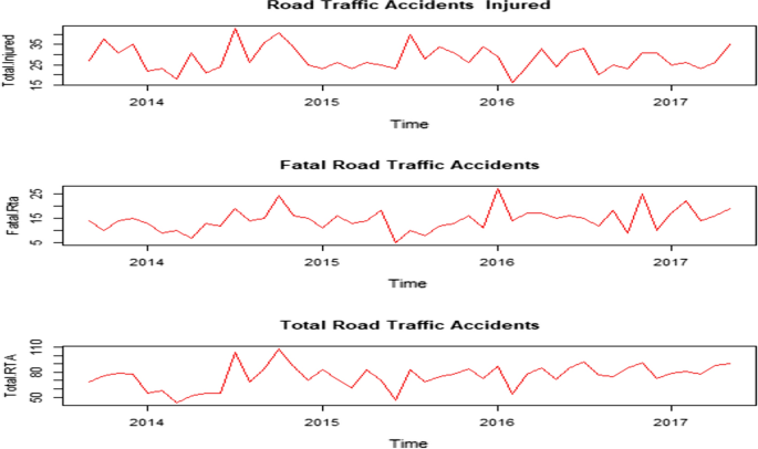
Time series plots of the injury cases, fatal RTA cases, and total RTA cases are shown below.

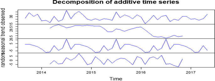
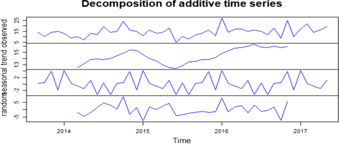
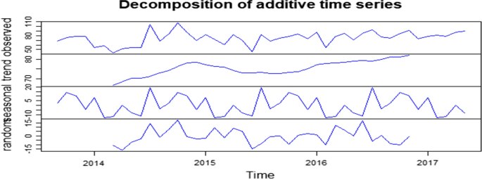
We can’t infer from the time series plot shown in Fig. 1 that the trend of the data since the graphs didn’t show clear patterns. There is a need for further analysis to find out the exact non-stationary and seasonality in the data. As shown from the time series decomposition plots (Figs. 2, 3, 4), the observed injury RTA cases show an overall decreasing trend whereas fatal RTA cases and total RTA cases have an overall increasing trend.

Fig. 1

Time series plot of monthly reported Injury, fatal and total road traffic accidents in Amhara Region (September 2013 to May 2017)

Fig. 2

Time series decomposition of injury RTA data

Fig. 3

Time series decomposition of fatal RTA data

Fig.4

Time series decomposition of Total RTA data

Test of stationarity

To test the stationarity of the data Augmented Dickey-Fuller test for stationarity was used. According to the ADF-test output in Table 4, fatal RTA and Total RTA data are not stationary. Only the injury RTA data is shown to be stationary since it has a p-value less than 0.05. Therefore, according to the Adf-tets statistics shown in Table 5 the fatal RTA and Total RTA data should be differenced to achieve stationarity.

Table 4 Summary statistics for ADF test of stationarity

Table 5 Summary statistics for ADF test of stationarity after differencing

After applying the first-order differencing on fatal RTA and total RTA cases, it can be shown that both p-values of Adf-Test are small (less than 0.05) which suggests the data is stationary and doesn’t need further differencing.

Fitting time series models

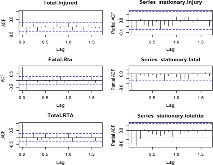
Once the data is ready and satisfies all the assumptions of modeling, the next step is to select the appropriate ARIMA model i.e., to determine the order of the model to be fitted. This task can be done by examining two important plots called autocorrelation function (ACF) and partial autocorrelation (PACF) plots of the stationary time series. For the current data, the PACF and ACF plots are shown below.

Model selection

The model selection was done by examining the ACF and PACF plots (Fig. 5). The AIC and BIC values are also used to choose the best model. These criteria are closely related and can be interpreted as an estimate of how much information would be lost if a given model is chosen. ARIMA [2] (1,0,0) [12], ARIMA (2,0,0) and ARIMA (2,0,0) (1,1,0) [12] are chosen as the best models for Total injury, Fatal RTAs and Total RTAs series respectively. As it is shown below in Table 6, the models  chosen above had the lowest AIC and BIC values compared with the other possible models.

Table 6 Parameter estimates & goodness of fit measures of injury, fatal and total RTA

Fig. 5

Autocorrelation and Partial autocorrelation function plots of Injury, Fatal and Total RTA

Model diagnostics

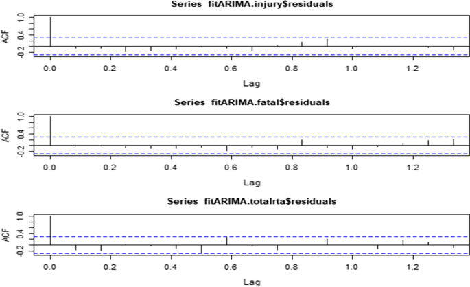
Now before using the fitted model for forecasting, one should examine the adequacy of the models. This can be commonly checked by examining ACF and PACF plots for model residuals. If model order parameters and structure are correctly specified, we would expect no significant autocorrelations present.

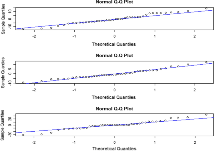
All standardized residuals plot shows no obvious trend and pattern and looks like an independent and identical distribution. Similarly, all plots of ACF residuals of the diagnostics show no evidence of significant correlation in the residuals. Most of the residuals are located on the straight line except for a few outliers deviating from the normality. In conclusion, the residuals ACF (Fig. 6) and normal Q-Q plots (Fig. 7) both exhibited a white noise pattern and the goodness of the fitted model.

Fig. 6

Diagnostics of residuals for ARIMA of injury, fatal, and total RTA data

Fig. 7

Normal Q-Q plot of residuals for ARIMA of injury, fatal and total RTA data

Forecasting

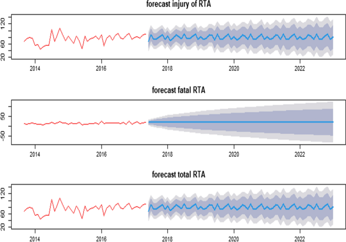
The model was fitted for 48 months period after the diagnostic test. The predicted counts of injury and total road traffic accidents for the mentiond forecast period are presented in Table 7. In addition, graph which gives a pictorial view of the observed series, its forecast, and confidence intervals of the forecasts are provided below.

Table 7 Predicted counts of injury and total road traffic accidents from June 2017 to May 2021

As it can be shown from the forecast plots (Fig. 8) as well as the table of predicted road traffic accidents, the trends of injury road traffic cases and total traffic cases generally exhibit a similar pattern with the observed data i.e., the situation keeps what it was before. This result signifies the cases will remain unchanged for the coming 48 months unless new or improved road safety measures are taken. It is in line with what we observe in our day-to-day life that road traffic accidents are common cases here and there.

Fig. 8

Graph of injury, fatal, and total RTA cases, its forecasts, and confidence intervals

Discussion

Nowadays, the increment of a road traffic accident at a disturbing rate is a major concern in Ethiopia. The current study focuses on the Amhara region which has the highest share of road traffic accidents in the country. The most widely used conventional method of time series is known as Autoregressive Integrated Moving Average (ARIMA) model, also known as the Box-Jenkins method was applied to monthly reported road traffic accident data in four randomly selected zones of the Amhara region from September 2013 to May 2017 to determine patterns of road traffic accident cases in the region. After identifying various tentative models, the appropriate models for the accident cases (Total injury, fatal and total road traffic accidents) are as follows. ARIMA (2,0,0)(1,0,0)[12], ARIMA(2,0,0) and ARIMA(2,0,0)(1,1,0)[12] are chosen models to model the total injury cases, fatal cases and total RTA cases using the data from September 2013 to May 2017. The adequacies of the model were tested by analyzing standard residuals in different forms. 48 months of forecasts were provided for injury cases, fatal cases and total cases would continue in a non-decreasing trend. This study provides reliable and genuine information that could be useful for determining road accident rates in the region supported by [18]. This study would also be used for providing important information to increase the level of awareness among stakeholders concerning road safety since the problem has become a growing issue in the country as a whole. Most importantly, this study would provide expected benefit to the road users, Road Safety Authority, researchers, and other stakeholders in understanding the rate of the cases of a road accident.

Conclusion

Based on the results of this study, the rate of road accidents is expected to remain constant for at least the next 4 years. It was found that the incidence of road accidents in the Amhara region can be fitted ARIMA(2,0,0)(1,0,0)12 and ARIMA(2,0,0)(1,1,0)₁₂ model. The findings of this study draw attention to the importance of implementing key road safety measures to change the existing threat of road accidents in the Amhara region. Therefore, improved and better policies of the National road safety authority should be introduced with much emphasis on publication and education to ensure a maximum reduction in Road accident crashes.

References

Farag SG, Hashim IH, El-Hamrawy SAJIJTTE. Analysis and assessment of accident characteristics: Case study of Dhofar Governorate, Sultanate of Oman. Int J Traffic Trans Eng. 2014;3:189–98.
Global status report on road safety. Accident: WHO; 2018. https://knoema.com/WHOGSRS2019Jan/global-status-report-on-road-safety-2018?country=1001720-ethiopia.
Bjerre J, Kirkebjerg PG, Larsen LB. Prevention of traffic deaths in accidents involving motor vehicles. Ugeskr Laeger. 2006;168(18):1764–8.
Smart RG, Mann RE. Deaths and injuries from road rage: cases in Canadian newspapers. CMAJ. 2002;167(7):761–2.
Peden M. Global collaboration on road traffic injury prevention. Int J Injury Control Safety Promotion. 2005;12(2):85–91.
Bishai D, Quresh A, James P, Ghaffar A. National road casualties and economic development. Health Econ. 2006;15(1):65–81.
Astrom J, Kent M, Jovin R. Signatures of four generations of road safety planning in Nairobi City, Kenya. J Eastern Afr Res Dev. 2006;20:186–201.
World Health Organization. Road traffic injuries. 2020. https://www.who.int/news-room/fact-sheets/detail/road-traffic-injuries.
Mariam DH. Road traffic accident: a major public health problem in Ethiopia. Ethiopian J Health Dev. 2014;28(1):1–2.
Persson A. Road traffic accidents in Ethiopia: magnitude, causes, and possible interventions. Adv Transportation Studies. 2008;15:5–16.
Organization WH. Global status report on road safety 2015. World Health Organization; 2015.
Association EE. Energy, safety, and environment and transport services in Ethiopia. Research Brief. 2012(2).
Johansson P. Speed limitation and motorway casualties: a time series count data regression approach. Accid Anal Prev. 1996;28(1):73–87.
Nihan NL, Holmesland KO. Use of the Box and Jenkins time series technique in traffic forecasting. Transportation. 1980;9(2):125–43.
Box GE, Jenkins GM, MacGregor JF. Some recent advances in forecasting and control. J R Stat Soc Ser C. 1974;23(2):158–79.
Box GE, Jenkins GM. Time series analysis: forecasting and control San Francisco. Calif: Holden-Day; 1976.
Twenefour FB, Ayitey E, Kangah J, Brew L. Time series analysis of road traffic accidents in Ghana. Asian J Probab Stat. 2021. https://doi.org/10.9734/AJPAS/2021/v11i230262.
Al-Ghamdi AS. Time series forecasts for traffic accidents, injuries, and fatalities in Saudi Arabia. J King Saud Univ Eng Sci. 1995;7(2):199–217.
Acknowledgements
The author would like to acknowledge the Amhara region police commission traffic departments, transport, and communication bureau to conduct this study and to publish this paper.
Funding
No funding was received for this study.
Author information
Authors and Affiliations
Contributions
KAG was responsible for the formulation of the methodology. KAG made substantial contributions to the conception and design of the study, analyzed and interpreted the data, and was a major contributor in writing the manuscript. KAG drafted the manuscript. All authors read and approved the final manuscript.
Corresponding author
Ethics declarations
Ethics approval and consent to participate
Not applicable.
Consent for publication
Competing interests
The authors declare that they have no competing interests.
Additional information
Publisher's Note
Springer Nature remains neutral with regard to jurisdictional claims in published maps and institutional affiliations.
Rights and permissions
Open Access This article is licensed under a Creative Commons Attribution 4.0 International License, which permits use, sharing, adaptation, distribution and reproduction in any medium or format, as long as you give appropriate credit to the original author(s) and the source, provide a link to the Creative Commons licence, and indicate if changes were made. The images or other third party material in this article are included in the article's Creative Commons licence, unless indicated otherwise in a credit line to the material. If material is not included in the article's Creative Commons licence and your intended use is not permitted by statutory regulation or exceeds the permitted use, you will need to obtain permission directly from the copyright holder. To view a copy of this licence, visit http://creativecommons.org/licenses/by/4.0/.
About this article
Cite this article
Getahun, K.A. Time series modeling of road traffic accidents in Amhara Region. J Big Data 8, 102 (2021). https://doi.org/10.1186/s40537-021-00493-z
Received:
Accepted:
Published:
DOI: https://doi.org/10.1186/s40537-021-00493-z