A comparative dimensionality reduction study in telecom customer segmentation using deep learning and PCA

Abstract

Telecom Companies logs customer’s actions which generate a huge amount of data that can bring important findings related to customer’s behavior and needs. The main characteristics of such data are the large number of features and the high sparsity that impose challenges to the analytics steps. This paper aims to explore dimensionality reduction on a real telecom dataset and evaluate customers’ clustering in reduced and latent space, compared to original space in order to achieve better quality clustering results. The original dataset contains 220 features that belonging to 100,000 customers. However, dimensionality reduction is an important data preprocessing step in the data mining process specially with the presence of curse of dimensionality. In particular, the aim of data reduction techniques is to filter out irrelevant features and noisy data samples. To reduce the high dimensional data, we projected it down to a subspace using well known Principal Component Analysis (PCA) decomposition and a novel approach based on Autoencoder Neural Network, performing in this way dimensionality reduction of original data. Then K-Means Clustering is applied on both-original and reduced data set. Different internal measures were performed to evaluate clustering for different numbers of dimensions and then we evaluated how the reduction method impacts the clustering task.

Introduction

Due to the increased competition between telecommunication operators and growing customers’ churn rate, telecommunication companies were seeking to improve customer loyalty. In order to increase customer satisfaction, most telecom companies resort to customer segmentation which entails separating the targeted customers into different groups based on demographics or usage perspective including gender, age-group, buying behavior, usage pattern, special interests and other features that represent the customer. Customer segmentation adopted by most telecom operators to provide the customer with the right offer.

Clustering high dimensional data

Data dimensionality in statistics refers to how many attributes a dataset has. Big data is one of the most common topics in present studies, and its techniques are applied in different fields such as telecom industry [1] to support strategic decisions. Clustering involves the grouping of similar objects into a set known as cluster. Objects in one cluster are likely to be different when compared to objects grouped under another cluster, and it’s one of the most fundamental processes for analyzing unsupervised data, which is applied in a wide range of applications such as computer vision [2,3,4], natural language processing [5,6,7] and bioinformatics [8, 9]. Many algorithms have been suggested over the previous eras to address clustering issues [10, 11]. There are two famous feature-based techniques among the current algorithms, K-means [12] and Gaussian Mixture Models (GMM) [13]. K-means makes it difficult to cluster each sample to its closest cluster center. A Gaussian mixture model is a probabilistic model that assumes all the data points are generated from a mixture of a finite number of Gaussian distributions with unknown parameters and attempts to infer distribution of the data.

Learning from large amount of data is a very challenging issue that faces most of feature-based clustering and other data analysis techniques, as data analysis becomes more difficult due to the “curse of dimensionality” [14]. So, high-dimensional data processing requires using proper techniques and methods [15]. The objective of dimensionality reduction methods is to learn an appropriate and simplified data representation from the original dataset [16,17,18] in order to get more insight from huge data. While many approaches have been presented to handle the challenges of reducing dimensionality and clustering, standard clustering techniques generally have bad efficiency on high-dimensional data because of the inefficiency of similarity measures used in them. In addition, using these techniques with large-scale datasets usually suffer from high computational complexity. For this purpose, techniques for reducing dimensionality and transforming features have been widely researched to map the raw information into a new feature space where clustering algorithms and data analysis techniques can be applied on representative features instead of the entire feature space. Generally, current techniques of data transformation include linear transformation such as Principal Component Analysis (PCA) [19] and non-linear conversion such as kernel methods [20], spectral methods [11] and deep learning-based techniques which have shown an impressive result in eliminating irrelevant and redundant information. Encouraged by a serious interest in deep learning, many researchers use autoencoders [21] and clustering approaches to address the objective of data representation and clustering.

Deep Autoencoder: challenges and issues

Deep learning is a subset of machine learning in artificial intelligence (AI) that has networks capable of learning unsupervisedly from unlabeled data by working with multi-level learning of data representations [22] Recently, Deep learning has been applied successfully in many fields, such as image classification and speech recognition [23] because these deep architectures can automatically learn features from images, sound or text data. Deep neural networks (DNNs) can be used to transform the raw data into more cluster-friendly representation through high-level non-linear mapping [24]. Due to the advancement of deep learning [25] including autoencoder (AE) algorithm and its deep version (DAE), deep embedding clustering (DEC) [26], followed by other novel methods [27, 28] are proposed. Which use deep representation to improve clustering performance. Autoencoders [21, 29] are considered an unsupervised learning technique and a specific form of feedforward neural networks where the input is the same as the output. They compress the input into a lower-dimensional code and then reconstruct the output from this representation. The code is a compact “compression” of the input, also called the latent-space representation, the training process is still based on the optimization of a reconstruction error or loss function. An autoencoder consists of three components: encoder, code and decoder. The encoder compresses the input and produces the code, the decoder then reconstructs the input only using this code as shown in Fig. 1. An autoencoder can learn a representation or encodes the input features for the purpose of dimensionality reduction. If linear activations or a single hidden layer of sigmoid are used, then the ideal solution for an autoencoder is heavily linked to Principal Component Analysis (PCA). Autoencoders can learn data projections with suitable dimensionality and sparsity limitations that are more useful than other fundamental methods such as PCA which only allow linear data transformation. on the other hand, autoencoders are non-linear and can learn more complicated relations between visible and hidden units. They can also be stacked, which makes them even more powerful. A number of works have recently covered clustering approaches that combine classical clustering algorithms with techniques of deep learning. These methods either follow a sequential approach where a deep representation is learned using a deep autoencoder [7, 30,31,32,33,34] before clusters are obtained using clustering method (e.g. k-means). or a simultaneous approach which use deep neural networks to simultaneously learn features representations and cluster assignments by optimizing a single objective function [35, 36]. Both approaches enhance efficiency in clustering. However, when dealing with real-world data, current clustering algorithms based on deep autoencoders have major drawbacks that restrict their reliability and ease of use, such as, initialization of the weights that is initializing the weights with random values clearly adds randomness to the obtained results [37] and the network architecture (or structure) (i.e. number and width of layers) which forces the network to obtain a different representation of the data while keeping important information. However, most of the recent researches on deep clustering [35, 36, 38,39,40] proposed a different structure for each studied dataset and the clustering efficiency of the techniques proposed strongly depends on a specific DAE structure.

Fig. 1

Schema of Autoencoder architecture

The contributions of our work and structure

The goal of this paper is to perform feature selection and high dimensional data reduction with different techniques to examine their performance in telecom customer segmentation as case study.

More in detail, three scenarios will be compared, which are the data set without performing any feature reduction, the data set preprocessed by feature reduction using PCA only, and the data set preprocessed by data reduction using Autoencoders to perform representation learning which enhances the customer segmentation model in terms of both accuracy and running time or mitigates constraints evaluated on high dimensional data. In this case study, we use sequential clustering approach starting with applying data reduction using a fully convolutional autoencoder to learn clustering-friendly representations of the data and it is trained with the standard mean squared error then perform clustering on the represented dataset then comparing the results with standard clustering after reducing the dimensionality linearly with PCA. The rest of this paper is structured as follows: the related work is presented in “Related work” section. “Research methodology” section we review our dataset for which no classical methods are well adapted and suggest our research methodology including the data transformation, correlation analysis and the use of Deep Clustering algorithm along with its results. In “Results and discussion” section, we discuss the evaluation of the suggested techniques and compare the efficiency of sequential and simultaneous clustering methods in our case, whereas the paper is concluded in “Conclusion and future work” section along with shedding light on future perspectives.

Related work

Companies using customer segmentation technique because each client is distinct and their marketing efforts would be better by building an efficient marketing and business strategies. Companies also hope to obtain a deeper understanding of the preferences and needs of their customers, with the concept of finding out what each segment finds most useful to tailor marketing products to that segment more correctly [41]. More recently, many techniques of customer segmentation in telecom sector have been proposed because of the increased amounts of data passing through various communication channels that make old techniques and methods no longer applicable. However, several researches in high dimensional data spaces have been studied. We highlight these works in this section briefly and review the clustering of high-dimensional data.

A Vodafone Case Study by Jansen proposed a customer segmentation and profiling model based on call usage behavior [42]. Twelve features are used as a summary description of customers and to build customer segments based on their incoming and outgoing calls over the time period P such as (average call duration, average calls received per day, average calls received per day, daytime calls… etc.). Each segment describes a certain behavior of customer’s group. A customer’s segment was estimated based on the customer’s profile using the data mining technique called Support Vector Machines. Two solutions have resulted from customer segmentation, the first is four segments and the second is six segments. With the Support Vector Machine approach, 80.3% of the cases classified the segment of a customer correctly, based on its profile for the situation with four segments. With six segments, the correct classification of 78.5% is obtained. Aheleroff et al. [43] used data set containing Call Detail Record (CDRs) of a mobile operator, located in the Middle East that has about 35 million mobile subscribers to categorize the subscribers into four loyal groups based on the level of customer’s loyalty during their life cycle. The usage patterns are obtained from detailed call/event records based on mobile services such as GPRS/MMS–SMS, including main usage information such as (incoming call number, outgoing call number, call time and date, call duration, call type, location…) which selected as the core items to monitor customer’s behavior. Then they Applied k-means as a well-known segmentation algorithm. The suggested customer life cycle model considered the past contribution, potential value, and churn probability at the same time. After identification of subscriber’s behavior and loyal group, the output customers’ clusters are used to make an applicable strategic plan for each group to improve customer satisfaction. While Masood, Salar, et al. [44] used a real customer data of a telecommunications company of Pakistan to apply a two-step clustering algorithm based on the call usage, revenue and recharge analysis, they made five revenue segments, that each one was further segmented based on user’s call usage data. The customers were segmented based on their revenue attributes such as Final Revenue, Calls Revenue, SMS Revenue and Value Added Services (VAS) Revenue. The number of clusters was manually selected as five, because the value for silhouette measure of clusters (which indicates the quality of clustering result as poor, fair or good) found to be more than 0.5 which shows that good clustering has been done by the algorithm. The two-step clustering algorithm was applied, first step all the cases are assigned to pre-clusters, During the second step, these pre-clusters are handled as individual cases and are further clustered using the hierarchical clustering algorithm, the results were thoroughly analyzed. It was shown that VAS usage was greater than the SMS usage for all customers’ segments. Every cluster was analyzed to uncover its call as well as SMS usage behavior. Most of the previous studies built their models based on a few number of features. Classical approaches for reducing dimensionality, such as Principal Component Analysis (PCA), were widely considered for the task of embedding. The linear nature of such methods, however, makes it difficult to infer true depictions of real-world data, typically based on extremely non-linear manifolds. This motivates research into profound learning models (e.g. auto-encoders, convolutional neural networks) that have been shown to be effective in extracting highly non-linear characteristics from complex data such as text, images, or graphs [21, 22, 29]. Deep autoencoders (DAE) have been shown to be helpful in reducing dimensionality [21] and denotation images. The autoencoders (AE) in specific can represent data into a new space in a non-linear manner. Related to clustering, the general idea is to represent the data into a low dimensional space by encoding only the most relevant information that characterizes the original data, reducing noise and sparsity, and then perform clustering in this new space. Recently, several notable works have mixed embedding learning and clustering. The suggested techniques usually perform both clustering and deep embedding in two different ways. First, some works suggested a sequential combination of deep embedding and clustering. In [30] the researchers use a stacked autoencoder to learn a representation of the affinity graph and then apply K-means to get the clusters on the learned representations. More lately, [45] suggest to include an autoencoder within the context of Deep Embedded Clustering (DEC) [26]. Then, together with local structure conservation, the suggested framework can perform clustering and learn representative characteristics. Additionally, a new technique to perform non-linear reconstruction has been suggested in [46] to adopt deep neural networks for representation-based community detection. Several researches recommend performing both the embedding process and the clustering task jointly in order to allow clustering to control the features extraction and vice versa. As an example in [36] a general framework, known as DeepCluster was proposed, to combine traditional clustering methods [K-means and Gaussian Mixture Model (GMM)] into deep learning models and adopt Alternating Direction of Multiplier Method to optimize it, the Performance was compared on the three real datasets (MNIST, USPS and Reuters10K), The highest values of all metrics on the datasets were belonged to the proposed DeepCluster framework.

Research methodology

This section describes the data set used in this work including features extraction as well as steps of clustering high dimensional data process presented in Fig. 2.

Fig. 2

Steps of clustering process

Input data and preparation

Our segmentation model inputs are based on mobile users’ actions or events over Syrian society. Four main sources of data are available in more detail: Call Detail Records (CDR), Database of Cell Towers, Customer’s services and Customers’ contract information.

Features extraction

The accuracy of segmentation relies mainly on the selection of features and the technique of segmentation. For customer segmentation problem, the features mainly come from the data gathered in the enterprise database, after being extracted from various resources. However, feature extraction [47] is the process of transforming the input data into a set of features which can very well represent the input data. The feature extraction process is done depending on our research goal using in memory-processing tools for processing and analytical purposes. The extracted features are categorized as follows: (some features may belong to more than one category):

• 1. The behavioral features which could be classified into individual, spatial, and social network features as follows:

  • Individual features describe the mobile phone usage and interactions of an individual with contacts. (e.g. average call duration per day, standard deviation of received SMS per day at worktime, the response rate of the user). Individual behavioral features are extracted from Call Detail Records (CDRs) generated by the Syrian Telecom cellular network. CDRs log the users’ activities for billing purposes and network management.

  • Spatial features describe the mobility patterns of an individual during the usage of mobile phone (e.g. entropy of visited antennas, average of mobility, daytime antenna entropy). Spatial and mobility features are extracted based on the database of cell towers and their locations as Table 1.

    Table 1 Sample of cells and sites database

  • Social network features describe the social network of an individual and compare their behavior with that of their peers. (e.g. clustering coefficient, assortativity).

  The extracted behavioral features are about (200) features related to the previous three categories and the rest of features are extracted from another sources. Table 2 shows a sample of extracted behavioral features.

  Table 2 Sample of behavioral extracted features

• 2. Customer’s subscribed services All services that the client enrolled in have been gathered and categorized manually on the basis of the type of service, such as services related to s bundles subscription, etc…, these categories are handled as customer features. As a result we got Table 3 of customer’s service.

  Table 3 Sample of customer’s services

• 3 Customer’s demographic data reflect some basic states of customer. Such as customer’s name, address, age, sex and details of client subscriptions as number (two or more GSMs) and types of subscriptions: pre-paid, post-paid, 3G, 4G… are extracted from the customers’ contract data and considered as additional features.

  We build and train the model using records related to 100,000 subscribers within about 6 months, with over 220 different features derived from CDRs, subscription information and registered services for each customer in our case study. Our goal is to take benefit of all features by reducing the dimensions, in order to filter out irrelevant features and noisy data samples.

The experimental process

Data extracted from the source location is often not usable in its original form. To overcome this obstacle, raw data must be transformed into a useful and efficient format, in our case study data is cleansed first before it can be transformed as follows: this work includes different stages (data exploration, features extraction and selection, and model validation), however different machine learning methodologies is used:

• Data cleansing, Data is cleansed through processes such as filling in or removing missing values, smoothing the noisy data, or resolving the inconsistencies in the data.

• Data transformation, standardization is the key pre-processing step in data mining to standardize features or attributes values from different dynamic ranges to a specific range. Applying standardization step leads to obtain better quality, efficient and accurate clustering results. It is also important to select a specific standardization procedure, according to the nature of the datasets for the analysis [48]. In our case, the result obtained by the z-score standardization method where it is more efficient than other standardization methods. Min-Max scaling is typically done via the following formula:

  $$\begin{aligned} MinMax{\text{-}}score= & {} \frac{x-\min (x)}{\max (x)-\min (x)} \end{aligned}$$

  (1)

  In Z score normalization, we perform the following formula:

  $$\begin{aligned} Z{\text{-}}score= & {} \frac{x-\mu }{\sigma } \end{aligned}$$

  (2)

  where is the mean of the population, is the standard deviation of the population.

  Min–Max scales the values closer to mean. But when data outliers are important and we don’t want to lose their impact, we attempt to scale with Z score normalization.

• Dimensionality reduction, dimensionality is the number of characteristics, variables, or features that describe the dataset. These dimensions are represented as columns and the goal is to reduce their number. In most cases, those columns are correlated and therefore, there is some information that is redundant which increases the dataset’s noise. This redundant data has a negative impact on the results of training our model and therefore it’s important to use dimensionality reduction techniques such as Feature Selection and Feature Extraction as a very useful way to reduce the model’s complexity and avoid overfitting. In our case study, we applied three different scenarios which lead to different clustering models, shown in Fig. 3, described as follows:

  • 1. The baseline this process is to perform clustering on the original data set without performing any data reduction method. Therefore, the comparison between the results allows us to understand whether the reduced data sets can make the clustering accuracy better than the result without performing data reduction.

  • 2. (PCA–based) customer segmentation

    First, the PCA transformation is applied to the original data. Data is transformed into new features as a combination of the original features in a new space, compressed in a way that the most relevant information is retained. Then, k-means clustering algorithm was applied on the transformed dataset.

    However, applying PCA before clustering is a powerful method for clustering high dimensional data in the presence of the linear correlations in features. So, we would like to know which feature reduction method can enhance the clustering accuracy.

    Step1: PCA implementation Using unlabeled training dataset, we actually have a data matrix X of 100,000 × 220. The matrix representation of the information not only makes the variables difficult to visualize and interpret but also computationally taxable when perform clustering. Therefore, we apply PCA to reduce the dimensionality of the data by finding projection direction(s) that minimizes the squared errors in reconstructing the original data or equivalently maximizes the variance of the projected data. Its performance depends on the distribution of the data set and the correlation of features.

    PCA is mathematically defined as an orthogonal linear transformation that transforms the data to a new coordinate system such that the greatest variance by some projection of the data comes to lie on the first coordinate (called the first principal component), the second greatest variance on the second coordinate, and so on. The first step of PCA is to standardize the dataset matrix. That’s important because features or columns with larger scales compared to other columns will ultimately dominate the final principal component matrix, i.e. attributing most of the explained variance to these features. This step is performed by Standard Scaler which subtracting each column mean from each column and dividing by their respective standard deviation. However, standardization has other advantages, such as faster learning for neural networks, which will later become important when autoencoder is implemented. The second step is to calculate the covariance matrix of the standardized matrix. The covariance between the variables can be found by performing matrix multiplication between the standardized matrix and its transposition, the result matrix should be a 220 × 220 symmetric matrix. where each diagonal element is the variance of each feature and every non-diagonal element is a particular co-variance between two features. Therefore, the covariance matrix, will have the following structure:

    $$\begin{aligned} Cov{\text{-}}Matrix = \begin{bmatrix} var(x1) &{} cov(x1,x2) &{} \dots &{} cov(x1,x220) \\ cov(x1,x2) &{} var(x2) &{} \dots &{} cov(x2,x220) \\ \vdots &{} \vdots &{} \ddots &{} \vdots \\ cov(x1,x220) &{} cov(x2,x220) &{} \dots &{} var(x220) \end{bmatrix} \end{aligned}$$

    The third step is to discover the covariance matrix’s eigenvectors using eigenvalue decomposition to get a matrix whose columns are Cov-Matrix’s eigenvectors. The eigenvectors matrix has columns that representing the principal components (the new dimensions), each component is orthogonal to each other and arranged in decreasing order of explained variance.

    The last step is to use the transformation matrix (eigenvectors matrix), by multiplying it with the scaled data matrix to compute the principal component scores in order to find the optimal number of components which capture the greatest amount of variance in the data.

    In our analysis, the applied method to determine the number of principal components is to look at a Scree Plot, which is the plot of the principal components ordered from largest to the smallest. The number of components is determined at the variance drop-off point where the gain in explained variances first decreased significantly, beyond which the remaining eigenvalues are all relatively small and of comparable size [49].

    As shown in Fig. 4, a Scree plot with bars displaying the explained variance as a percentage of total variance by the first 20 PCs such that 90% of the variance is retained and showing variance drop-off after the third component account for roughly 28% of the total explained variance.

    We found that, the first three principal components explain 72% of the variation. This is an acceptably large percentage. Assume that the transformation matrix as TM-L, when reducing the dimensionality of our dataset, where L is the number of principal components such that $\hbox {L}<220$. We can then compress the data using TM-L, where TM-L still has the same number of rows but only L columns, leading to a reduced dataset on which the clustering Algorithm is applied in an unsupervised manner, since we don’t have labels, but it’s important to reveal the contributions of each feature on the components and then proceed to the last step in the process.

    After applying the PCA on the original data, we conducted our experiments on the principle components (10, 20, 30, 50) that maintain the largest percentage of variance in the data and give a total variance ratio greater than 80%, we evaluated the projection loss by calculating the MSE loss function which (expresses the difference between the reconstructed data from the projected data and the original data), obtained in Table 4.

    Table 4 The projection loss of the principal components

    Step 2: Reveal the most important variables/features after a PCA analysis, The important features are those that influence the Principle components more, and therefore have a high absolute value score on them. As a way to get how components are correlated with the original features we retrieve the indexes of the most important features on each component, the large value of the contribution means that the variable contributes more to the component and it is crucial in explaining the variety in the data set.

    Variables that don’t correlate with any component or correlated with the last dimensions are variables with low contribution and might be eliminated to simplify the overall analysis.

    The importance of each feature is reflected by the magnitude of the corresponding values in the eigenvectors. First, we get the amount of variance that each PC explain using (pca explained variance ratio) then we find the most important features. To sum up, we look at the absolute values of the Eigenvectors’ components corresponding to the k largest Eigenvalues. In sklearn the components are sorted by explained variance. The larger they are these absolute values, the more a specific feature contributes to that principal component. Table 5 describes the variables according to their contributions to the principal components expressed in percentage.

    So, for each principal component we can see which variables contribute most to that component as Table 6.

    Table 5 Variables contributions to the principal components

    Table 6 The most important features for each component

    Step 3: Find the Clusters, K-Means clustering algorithm is applied in this step to cluster the reduced dataset represented by top 20 PCs as new feature space. First, we applied the elbow method to determine the optimal number of clusters for k-means clustering.. for PCA, the k-means scree plot below in Fig. 5

    The Elbow Method is one of the most popular methods to determine this optimal value of k. The idea of the elbow method is to run k-means clustering on the dataset for a range of values of k (say, k from 1 to 15 in our case), and for each value of k calculate the sum of squared errors (SSE). Then, plot a line chart of the SSE for each value of k. If the line chart looks like an arm, then the “elbow” on the arm is the value of k that is the best. The idea is that we want a small SSE, but that the SSE tends to decrease toward 0 as we increase k (the SSE is 0 when k is equal to the number of data points in the dataset, because then each data point is its own cluster, and there is no error between it and the center of its cluster).So our goal is to choose a small value of k that still has a low SSE, and the elbow usually represents where we start to have diminishing returns by increasing k. Figure 5 shows

    An elbow chart showing the SSE after running k-means clustering for k going from 1 to 15. We see a pretty clear elbow at k = 4, indicating that 4 is the best number of clusters.

  • 3 (AutoEncoder-based) Customer Segmentation In addition to examine the model performance by linear transformation using PCA, dimensionality reduction based on Artificial Neural Network (ANN) is also considered. The result can be used to compare the performance of the autoencoder and PCA for the data reduction tasks.

    Autoencoders are generally a type of artificial neural network used for learning a representation or encoding of a set of unlabeled data as a first step towards reducing dimensionality by compressing (encoding) the input data matrix to a reduced set of dimensions and then reconstructing (decoding) the compressed data back to their original form. then the compressed data may be used in different applications such as clustering as our case.

    An autoencoder can learn nonlinear transformations using a nonlinear activation function and multiple hidden layers by taking an input layer (data matrix X), which is passed through hidden layers where their dimensions are lower than the input layer dimension to perform compression. The network aims to reconstruct the original data as close as possible to the original with minimum reconstruction error.

    Autoencoder training algorithm may be summarized in the following steps, for each input x:

    • 1. Feed-forward pass to calculate all hidden layers’ activations and store them in a memory cache-style. Simultaneously, calculate the final output x1 in the last layer.

    • 2. Measure deviation of x1 from input x using loss function.

    • 3. Backpropogate the error through the network and update the weights.

    • 4. Repeat until resulting loss is acceptable or other factor is satisfied.

    Step 1: Autoencoder Implementation For our experiments, we trained fully connected autoencoder as a symmetric model that is symmetrical about how the input data is compressed and decompressed by exact opposite manners.

    Before start training an autoencoder, it is essential to set our hyperparameters set including the model design components and training variables such as:

    • 1. Code size: the number of nodes in the middle layer. More compression results in smaller sizes.

    • 2. Number of layers: Represents the number of hidden layers needed for network training.

    • 3. Number of nodes per layer: With each subsequent layer of the encoder, the number of nodes per layer reduces and rises back into the decoder. In terms of layer structure, the decoder is symmetrical to the encoder.

    • 4. Loss function: represents the reconstruction error, either mean squared error or binary cross-entropy is used according to the input values if they are within [0, 1] then cross-entropy is typically used otherwise, the mean square error is used.

    • 5. Training variables: associated with the training process such as activation functions, learning rate, number of training epochs, batch size per epoch, as well as how often we want to display information about our training progress.

    We configure the Autoencoders using the Keras tensorflow with GPU support Python package, and compile the neural network with mean square error loss and Adam optimizer [50] with 0.001 learning rate and the default Keras parameters. We also set the number of training epochs to 200, While we set the batch size for the training cycle to 512.

    The size of our input is set to 220 neurons, which corresponds to our dataset’s number of features. We tried different hidden layer configurations as shown in Table 7; in order to minimize the reconstruction error computed by mean square error. All encoder/decoder pairs used rectified liner units (ReLU) activation function given in the following formula:

    $$\begin{aligned} f(x)= & {} \max {(0,x)} \end{aligned}$$

    (3)

    Table 7 Experimental results for different hidden layers configurations

    Following the training of the autoencoder while reconstructing the original data by encoding and decoding samples from the validation set, allows us to monitor training by TensorBoard web interface by plotting the Reconstruction Error (MSE) or loss function as seen in Fig. 6.

    Step 2: Clustering the Encoded dataset By training the autoencoder, we have its encoder part learned to compress each sample into 20 floating point values. We use k-means clustering Algorithm to perform clustering. To do this, we first fit the Encoded data to K-Means clustering algorithm and then determine the optimal number of clusters using Elbow method by measuring the sum of square distances to the nearest cluster center as Fig. 7.

  Fig. 3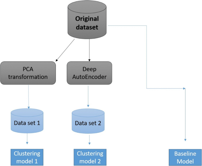

  

  The experimental process scenarios

  Fig. 4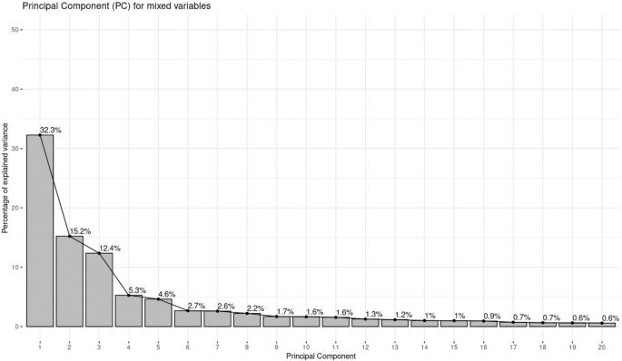

  

  Scree plot for the first 20 principal components

  Fig. 5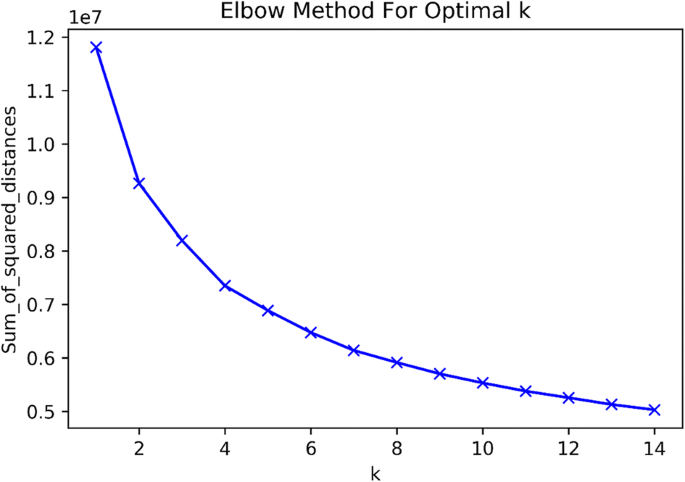

  

  Optimal number of clusters for PCA Reduced data

  Fig. 6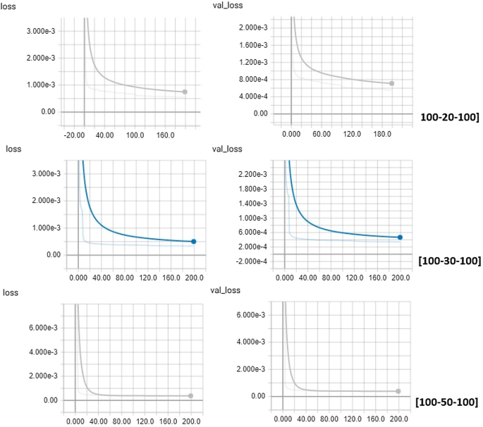

  

  Reconstruction Error (MSE)

  Fig. 7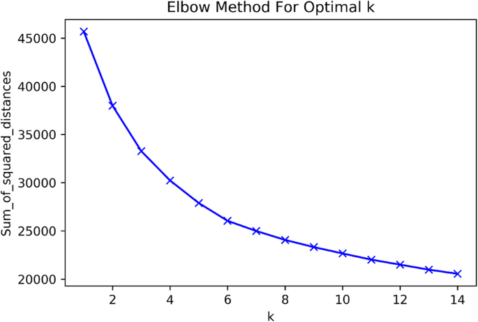

  

  Optimal number of clusters for Encoded data

Results and discussion

In this Chapter we introduce the obtained Clustering results for the reduced dataset with PCA transformation and Autoencoder Neural Network. After dimensionality reduction we performed K-Means clustering on the data with reduced set of features.

Clustering evaluation metrics

Different measures were performed for the final evaluation of the clustering algorithm performance, which can be categorized into 2 main types [51]:

• External cluster validation: comparing the results we got from cluster analysis to an externally known result, such as externally provided class labels. Since external validation measures know the right cluster number in advance, they are mainly used for choosing an optimal clustering algorithm on a certain data set [52].

• Internal cluster validation: which exploit the internal information of the clustering process to evaluate the performance of a clustering structure without depending on external information. also It can be used to estimate the appropriate and the better clustering algorithm without any external data [52].

In our research, we deal with unlabeled data so we review some internal measures that we can deploy on clustering algorithms to evaluate the quality of clustering results such as:

• Silhouette Coefficient The silhouette analysis measures how well the features are clustered and it estimates the average distance between clusters by measuring the similarity of an object is to its own cluster compared to other clusters. The values of the silhouette are ranged between − 1 and + 1, where the higher value of silhouette point out that the object is well matched to its own cluster and poorly matched to neighboring clusters and vice versa. The silhouette can be calculated with different distance metric, like the 1 Euclidean distance or the Manhattan distance. The silhouette analysis is calculated as below:

  $$\begin{aligned} S = \frac{1}{NC} \sum _{i} \frac{1}{ni} \sum _{x \in Ci} \frac{b(x) - a(x)}{\max [b(x),a(x)]} \end{aligned}$$

  (4)

• DB index The Davies–Bouldin index (DBI), an internal evaluation metric for evaluating clustering algorithms performance based on the average measure of similarity of each cluster with its most similar cluster where similarity is the ratio within-cluster distances to between-cluster distances. Lower the value of the DB index, clustering is better. It can be calculated for k number of clusters by the formula

  $$\begin{aligned} DBI = \frac{1}{k} \sum _{i=1}^{k} \max _{i \ne j}\left( \frac{\sigma i + \sigma j}{d(Ci,Cj)} \right) \end{aligned}$$

  (5)

  where Ci is the centroid of cluster i, is the average distance of all points in the cluster i to its centroid, d(Ci,Cj) is the distance between centroid Ci and Cj.

To obtain results we empirically set different parameters for our model, and evaluate its influence on our result. The tested Autoencoder network Architectures for our dataset has minimized the reconstruction error with 200 epochs and a batch size of 512 using Adam optimizer. The PCA algorithm has saved 90% of the variance with just 20 features which is a good reduction from our original space. We Applied K-Means clustering experiments with data set reduced to a different number of dimensions 20,30,50 features and also evaluated performance without dimensionality reduction to see how this parameter impacts the clustering task besides the reduction method. The mentioned metrics were used in this research to evaluate clustering on both original and the reduced data set. Figure 8 shows the average Silhouette score results for the reduced data set with PCA transformation and Autoencoder Neural Network Applied on 20, 30, 50 dimensions. Also, Fig. 9 shows the Davies–Bouldin scores obtained after applying K-Means Clustering on Reduced data to 20, 30, 50 dimensions using both of PCA and Autoencoder.

Fig. 8

Average Silhouette score with different dimensions

Fig. 9

Davies Bouldin score with different dimensions

There are several more ways to reduce the dimensionality, using PCA and autoencoders could be compared for a deeper understanding of their differences. Looking at the details of each approach’s loss function and how it evolves over time can provide extra information in the superiority of the neural network that generalizes better with so little training. As a result, Figs. 8 and 9 demonstrated that the best evaluation scores for this type of data was obtained by using autoencoder neural network for dimensionality reduction and K-Mean Clustering Algorithm, Silhouette score reached to 0.682 with 3 clusters and 0.571 with 5 clusters while the score obtained on the original data with 220 dimensions was 0.581 while the reduced dataset with PCA transformation achieved best 0.476 Silhouette score with 2 clusters. The experimental results indicated that our method is effective in the customer segmentation task and gave an idea why there was a need to move from PCA to autoencoders. Presenting the case for non-linear functions as compared to linear transformations as in PCA.

Given the simplicity of the autoencoder model used here, autoencoder significantly improved both of silhouette and DBI scores in our case study. What is remarkable also is that the best Average silhouette scores is related to the small numbers of clusters like 2 or 3 as shown in Fig. 10 that’s an indication to clustering algorithms works high performance whereas it produces more meaningful results with encoded data because the power of autoencoder to extract meaningful data,therefore most customers have similar behaviors and belong to 2 clusters.

Fig. 10

Average Silhouette Score for different Clusters

Conclusion and future work

The process of dimensionality reduction was performed using both PCA decomposition and Autoencoder Neural Network built with Keras TensorFlow model to perform clustering analysis with unlabeled datasets. k-Means Clustering algorithm was applied and evaluated on data in original and reduced space of features. Finally, we measured the effects of dimensionality reduction and compared two approaches, PCA and Autoencoder. The Clustering Performance was evaluated using Internal indices such as Silhouette index and Davies–Bouldin index. The best results for this type of data were obtained by autoencoder neural network approach which played a significant role in the dimensional reduction, and K-Mean Clustering Algorithm, where the clustering performance was enhanced with reduced dimensions. For the original data set of 220 features we were able to reduce its dimension to 20 features and obtain results very close or better than original dataset clustering evaluation results. Finally, while a neural network-style encoder performed better with clustering customers in our case study, it may not always be the case that an autoencoder can outperform a PCA representation of the data. If a linear map can sufficiently explain the variance in the data without significant loss of detail, then a neural network may be overkill when a simpler model like PCA can be used effectively.

It’s known that PCA and Autoencoders share architectural similarities. But despite this, an Autoencoder by itself does not have PCA properties, e.g. orthogonality. So the incorporating of the PCA properties will bring significant benefits to an Autoencoder, such as resolving vanishing and exploding gradient, and overfitting via regularization. Based on this, properties that we would like Autoencoders to inherit are (Tied weights, Orthogonal weights, Uncorrelated features, and Unit Norm). As a future work, we can Tune and Optimize Autoencoder using PCA principles by building custom constraints for our Autoencoder for tuning and optimization.

References

Al-Zuabi IM, Jafar A, Aljoumaa K. Predicting customer’s gender and age depending on mobile phone data. J Big Data. 2019;6(1):18.
Joulin A, Bach F, Ponce J. Discriminative clustering for image co-segmentation. In: 2010 IEEE computer society conference on computer vision and pattern recognition. New York: IEEE; 2010. p. 1943–50.
Liu H, Shao M, Li S, Fu Y. Infinite ensemble for image clustering. In: Proceedings of the 22nd ACM SIGKDD international conference on knowledge discovery and data mining. Nwe York: ACM; 2016. p. 1745–54.
Wang R, Shan S, Chen X, Gao W. Manifold-manifold distance with application to face recognition based on image set. In: 2008 IEEE conference on computer vision and pattern recognition. New York: IEEE; 2008. p. 1–8.
Aggarwal CC, Zhai C. A survey of text clustering algorithms. Mining text data. Berlin: Springer; 2012. p. 77–128.
Beil F, Ester M, Xu X. Frequent term-based text clustering. In: Proceedings of the eighth ACM SIGKDD international conference on knowledge discovery and data mining. New York: ACM; 2002. p. 436–42.
Xu J, Peng W, Guanhua T, Bo X, Jun Z, Fangyuan W, Hongwei H, et al. Short text clustering via convolutional neural networks; 2015.
Tian K, Shao M, Wang Y, Guan J, Zhou S. Boosting compound–protein interaction prediction by deep learning. Methods. 2016;110:64–72.
Zhang R, Cheng Z, Guan J, Zhou S. Exploiting topic modeling to boost metagenomic reads binning. BMC Bioinform. 2015;16:2.
Dueck D, Frey BJ. Non-metric affinity propagation for unsupervised image categorization. In: 2007 IEEE 11th international conference on computer vision. New York: IEEE; 2007. p. 1–8.
Ng AY, Jordan MI, Weiss Y. On spectral clustering: analysis and an algorithm. In: Advances in neural information processing systems. MIT Press; 2001. p. 849–56.
Kanungo T, Mount DM, Netanyahu NS, Piatko CD, Silverman R, Wu AY. An efficient k-means clustering algorithm: analysis and implementation. IEEE Trans Pattern Anal Mach Intell. 2002;7:881–92.
Bishop CM. Pattern recognition and machine learning. Berlin: Sspringer; 2006.
Bellman RE. Adaptive control processes: a guided tour, vol. 2045. Princeton: Princeton University Press; 2015.
Tan P-N, Steinbach M, Kumar V. Introduction to data mining. Boston: Addison-Wesley Longman Publishing Co., Inc.; 2005.
Yamamoto M, Hwang H. A general formulation of cluster analysis with dimension reduction and subspace separation. Behaviormetrika. 2014;41(1):115–29.
Allab K, Labiod L, Nadif M. A semi-nmf-pca unified framework for data clustering. IEEE Trans Knowl Data Eng. 2016;29(1):2–16.
Allab K, Labiod L, Nadif M. Simultaneous spectral data embedding and clustering. IEEE Trans Neural Netw Learn Syst. 2018;29(12):6396–401.
Wold S, Esbensen KH, Geladi P. Principal component analysis; 1987.
Hofmann T, Schölkopf B, Smola AJ. Kernel methods in machine learning. Ann Stat. 2008;36:1171–220.
Hinton GE, Salakhutdinov RR. Reducing the dimensionality of data with neural networks. Sscience. 2006;313(5786):504–7.
Bengio Y, et al. Learning deep architectures for ai. Found Trends® Mach Learn. 2009;2(1):1–127.
Szegedy C, Liu W, Jia Y, Sermanet P, Reed S, Anguelov D, Erhan D, Vanhoucke V, Rabinovich A. Going deeper with convolutions. In: Proceedings of the IEEE conference on computer vision and pattern recognition; 2015. p. 1–9.
Bengio Y, Courville A, Vincent P. Representation learning: a review and new perspectives. IEEE Trans Pattern Anal Mach Intell. 2013;35(8):1798–828.
Schmidhuber J. Deep learning in neural networks: an overview. Neural Netw. 2015;61:85–117.
Xie J, Girshick R, Farhadi A. Unsupervised deep embedding for clustering analysis. In: International conference on machine learning; 2016. p. 478–87.
Li F, Qiao H, Zhang B. Discriminatively boosted image clustering with fully convolutional auto-encoders. Pattern Recognit. 2018;83:161–73.
Wang Z, Chang S, Zhou J, Wang M, Huang TS. Learning a task-specific deep architecture for clustering. In: Proceedings of the 2016 SIAM international conference on data mining. Bangkok: SIAM; 2016. p. 369–77.
Baldi P. Autoencoders, unsupervised learning, and deep architectures. In: Proceedings of ICML workshop on unsupervised and transfer learning; 2012. p. 37–49.
Tian F, Gao B, Cui Q, Chen E, Liu T-Y. Learning deep representations for graph clustering. In: Twenty-eighth AAAI conference on artificial intelligence; 2014.
Shao M, Li S, Ding Z, Fu Y. Deep linear coding for fast graph clustering. In: Twenty-fourth international joint conference on artificial intelligence; 2015.
Wang W, Huang Y, Wang Y, Wang L. Generalized autoencoder: A neural network framework for dimensionality reduction. In: Proceedings of the IEEE conference on computer vision and pattern recognition workshops; 2014. p. 490–7.
Huang P, Huang Y, Wang W, Wang L. Deep embedding network for clustering. In: 2014 22nd international conference on pattern recognition. New York: IEEE; 2014. p. 1532–7.
Leyli-Abadi M, Labiod L, Nadif M. Denoising autoencoder as an effective dimensionality reduction and clustering of text data. In: Pacific-Asia conference on knowledge discovery and data mining. Berlin: Springer; 2017. p. 801–13.
Yang B, Fu X, Sidiropoulos ND, Hong M. Towards k-means-friendly spaces: Simultaneous deep learning and clustering. In: Proceedings of the 34th international conference on machine learning, vol. 70. JMLR. org; 2017. p. 3861–70.
Tian K, Zhou S, Guan J. Deepcluster: A general clustering framework based on deep learning. In: Joint European conference on machine learning and knowledge discovery in databases. Berlin: Springer; 2017. p. 809–25.
Seuret M, Alberti M, Liwicki M, Ingold R. Pca-initialized deep neural networks applied to document image analysis. In: 2017 14th IAPR international conference on document analysis and recognition (ICDAR). vol. 1. New York: IEEE; 2017. p. 877–82.
Banijamali E, Ghodsi A. Fast spectral clustering using autoencoders and landmarks. In: International conference image analysis and recognition. Berlin: Springer; 2017. p. 380–8.
Wang S, Ding Z, Fu Y. Feature selection guided auto-encoder. In: Thirty-first AAAI conference on artificial intelligence; 2017.
Affeldt S, Labiod L, Nadif M. Spectral clustering via ensemble deep autoencoder learning (sc-edae); 2019. arXiv preprint arXiv:1901.02291.
Lai X-a. Segmentation study on enterprise customers based on data mining technology. In: 2009 first international workshop on database technology and applications. New York: IEEE; 2009. p. 247–50.
Jansen S. Customer segmentation and customer profiling for a mobile telecommunications company based on usage behavior. A Vodafone case study; 2007.p. 66.
Aheleroff S. Customer segmentation for a mobile telecommunications company based on service usage behavior. In: The 3rd international conference on data mining and intelligent information technology applications. New York: IEEE; 2011. pp. 308–13.
Masood S, Ali M, Arshad F, Qamar AM, Kamal A, Rehman A. Customer segmentation and analysis of a mobile telecommunication company of pakistan using two phase clustering algorithm. In: Eighth international conference on digital information management (ICDIM 2013). New York: IEEE; 2013. p. 137–42.
Guo X, Gao L, Liu X, Yin J. Improved deep embedded clustering with local structure preservation. In: IJCAI. 2017. p. 1753–9.
Yang L, Cao X, He D, Wang C, Wang X, Zhang W. Modularity based community detection with deep learning. IJCAI. 2016;16:2252–8.
Aparna U, Paul S. Feature selection and extraction in data mining. In: 2016 online international conference on green engineering and technologies (IC-GET). New York: IEEE; 2016. p. 1–3.
Mohamad IB, Usman D. Standardization and its effects on k-means clustering algorithm. Res J Appl Sci Eng Technol. 2013;6(17):3299–303.
Peres-Neto PR, Jackson DA, Somers KM. How many principal components? stopping rules for determining the number of non-trivial axes revisited. Comput Stat Data Anal. 2005;49(4):974–97.
Reddi SJ, Kale S, Kumar S. On the convergence of adam and beyond; 2019. arXiv preprint arXiv:1904.09237.
Charrad M, Ghazzali N, Boiteux V, Niknafs A. NbClust: an R package for determining the relevant number of clusters in a data set. J Stat Softw. 2014;61:1–36.
Liu Y, Li Z, Xiong H, Gao X, Wu J. Understanding of internal clustering validation measures. In: 2010 IEEE international conference on data mining. New York: IEEE; 2010. p. 911–6.
Acknowledgements
This research was sponsored by SyriaTel telecom Co. We thank Eng.Ibrahem Alzuabi big data head of section, SyriaTel D3M unit for great ideas, help with the data processing and their useful discussions.
Funding
The authors declare that they have no funding.
Author information
Authors and Affiliations
Contributions
MA-KH took on the main role so he performed the literature review, implemented the proposed model, conducted the experiments and wrote the manuscript. MJ and KJ took on a supervisory role and oversaw the completion of the work. All authors read and approved the final manuscript.
Corresponding author
Ethics declarations
Ethics approval and consent to participate
The authors Ethics approval and consent to participate.
Consent for publication
The authors consent for publication.
Competing interests
The authors declare that they have no competing interests.
Additional information
Publisher's Note
Springer Nature remains neutral with regard to jurisdictional claims in published maps and institutional affiliations.
Rights and permissions
Open Access This article is licensed under a Creative Commons Attribution 4.0 International License, which permits use, sharing, adaptation, distribution and reproduction in any medium or format, as long as you give appropriate credit to the original author(s) and the source, provide a link to the Creative Commons licence, and indicate if changes were made. The images or other third party material in this article are included in the article's Creative Commons licence, unless indicated otherwise in a credit line to the material. If material is not included in the article's Creative Commons licence and your intended use is not permitted by statutory regulation or exceeds the permitted use, you will need to obtain permission directly from the copyright holder. To view a copy of this licence, visit http://creativecommons.org/licenses/by/4.0/.
About this article
Cite this article
Alkhayrat, M., Aljnidi, M. & Aljoumaa, K. A comparative dimensionality reduction study in telecom customer segmentation using deep learning and PCA. J Big Data 7, 9 (2020). https://doi.org/10.1186/s40537-020-0286-0
Received:
Accepted:
Published:
DOI: https://doi.org/10.1186/s40537-020-0286-0