Learning in the presence of concept recurrence in data stream clustering

Abstract

In the case of real-world data streams, the underlying data distribution will not be static; it is subject to variation over time, which is known as the primary reason for concept drift. Concept drift poses severe problems to the accuracy of a model in online learning scenarios. The recurring concept is a particular case of concept drift where the concepts already seen in the past reappear as the stream evolves. This problem is not yet studied in the context of stream clustering. This paper proposes a novel algorithm for identifying the recurring concepts in data stream clustering. During concept recurrence, the most matching model is retrieved from the repository and reused. The algorithm has minimum memory requirements and works online with the stream. Some of the concepts and definitions, already familiar in concept recurrence studies of stream classification have been redefined for clustering. The experiments conducted on real and synthetic data streams reveal that the proposed algorithm has the potential to identify recurring concepts.

Introduction

In the real world, applications producing continuous high-speed data streams are ever-increasing. Mining information from data streams is challenging due to their infinite length and evolving nature. A dynamic change in the data distribution which makes the existing model unfit to represent the recent data is called concept drift. The mining algorithm should be able to detect such changes and update the model accordingly.

As the stream flows continuously, new concepts might develop due to changes in the data distribution, attributes might appear or disappear in the long run, and sometimes even new classes might emerge. Along with these kinds of changes, a concept already processed in the past can reappear after some time. Numerous real-world applications can be found like weather, fashion, and consumer habits etc. where the concepts recur when the corresponding contexts repeat.

Usually, when concepts drift, models are newly learnt. In other words, a model is generally associated with a concept, since it represents the relationship between the input variables and the target variable. The detection of recurring concepts will help to avoid re-learning of models already seen the past. The models saved in a repository can be reused in case of concept recurrence. Besides saving the effort of re-learning, this makes the adaptation fast. Another advantage of recurrence tracking is the creation of a 'history of concepts'. It helps to explore the pattern in recurrence and thereby enables the prediction of an upcoming concept [13, 38].

Clustering is an essential method of stream analysis, particularly useful for unsupervised learning. Though most of the clustering algorithms consider the stream to be evolving, they handle concept drift implicitly through the use of window models [10]. Similarly, concept recurrence is not yet studied in the stream clustering scenarios.

This paper proposes an algorithm that can handle recurring concepts in data stream clustering. Figure 1 shows the position of the presented work in the literature. It comes at the intersection of data stream clustering, drift detection and concept recurrence handling. As part of this work, experiments are conducted on two different kinds of learning strategies—fixed size window based learning and explicit concept drift detection. Since the concept recurrence in data stream clustering is not explored yet, there are many questions to be addressed.

• How concept recurrence can be identified in data stream clustering and how models can be stored and reused in case of recurrence?

• In most of the real-life applications with recurring concepts, there are hidden contexts associated to concepts and concept recurrence is caused by context re-appearance. How to identify the hidden context, save the context and record the relationship between concepts and contexts [12, 13, 16, 36, 37]?

• If concepts are recurring, will it be possible to predict an upcoming concept? What can be different methods adopted to predict a concept [21, 38]?

• In data stream clustering scenarios, how the performance or the quality of a concept recurrence algorithm can be measured. What is the strategy to be used for removing old models when memory constraints exist?

Fig. 1

The position of the research problem in the literature

Among these, we focused on the first question and on elaboration it leads to the following points.

• How can models be stored in a repository with a compact representation? It has to deal with the trade-off between memory requirements and the loss of details of the clusters.

• How recurring concepts can be identified in unsupervised learning.

• Concerning concept recurrence, what difference does it make when the drift is handled explicitly?

• How can the performance of the recurrence handling algorithm be assessed in data stream clustering?

The models are stored in a repository to reuse on successful detection of concept recurrence. The match is measured between the models in the repository and the data received recently. Since error based assessment of models is not possible, the clustering structure similarities are measured for recurrence detection in the proposed algorithm. Using Hellinger distance, the similarity between the probability distributions is also measured, and the same is used to depict the correctness of the algorithm in identifying recurring concepts.

Rest of this paper is organized as follows. Next section includes the details of related work in the literature. “Preliminaries” section provides a brief account of the preliminary information, followed by “The proposed algorithm” section, which describes the algorithm in detail. “Experiments” section describes the experiment settings and the datasets. “Results and discussion” section presents the results of the experiments. Finally, “Conclusion” section concludes the paper.

Related work

In data stream clustering, there are some crucial requirements to be considered like compact representation to consume minimum memory, quick and incremental processing of data and fast detection of outliers [4]. Many data stream clustering algorithms have been proposed in the literature [1,2,3, 5, 14, 39]. In this paper, CluStream [2] is used as the basic algorithm for clustering the streams.

CluStream uses k-means during its initialization and macro-clustering stages. The underlying assumption while using the k-means algorithm is that the value k is fixed and it is provided externally. Since the streams are evolving, it is quite unrealistic to set the value of k in the beginning. In literature, we can see papers which proposed this idea [3, 7, 9, 23]. The value of k is kept variable in the experiments done as part of this study. The Ordered Multiple Runs of k-Means (OMRk) algorithm [23] with Simplified Silhouette [27, 34] is used as the relative clustering validity criteria for deciding the best value of 'k'.

The literature proposes different approaches to handling concept drift. Window-based learning and forgetting, ensemble-based methods, and explicit drift detection are the possible approaches in treating concept drift [10, 13]. Two of these methods are considered in our learning algorithm—window-based learning and explicit drift detection. The window-based learning and forgetting method is known to be useful for abrupt forgetting [10, 17]. But precise drift detection helps in understanding the dynamics of the underlying process that generates the data and ensures fast adaptation to the changes [10]. Only a few papers in the literature [3, 24, 26, 28] discuss explicit drift detection in data stream clustering. Among these, ODAC [26] is an attribute-based stream clustering algorithm. The other three [3, 24, 28] propose Page-Hinkley test, a variant of Cumulative sum (CUSUM) [30] as the method to detect concept drifts. An ensemble-based method of drift detection and adaptation is discussed in [32]. It uses an ensemble of clustering trees (CTs) for classifying textual streams with drift. Since this paper deals with the classification problem, drift detection is done based on prediction error.

Tracking recurrent concepts is a familiar topic in stream classification. Rest of this survey concentrates on recurrence detection algorithms developed for stream classification [37], might be the first work in the literature that considers the problem of recurring concepts. This paper introduces FLORA family of algorithms to handle various aspects of concept drift, and FLORA3 deals with recurring concepts. It presents the method of storing old models in a repository for reuse in case of recurrence. After FLORA, we can see many algorithms which address the idea of concept recurrence. As stated in [10], these algorithms can be broadly classified into single model approaches [11, 13, 21, 36, 37] and ensemble-based approaches [12, 16, 38].

Recurrence detection algorithms generally have two-layer structure; with the basic stream learning in the first layer and the meta-learning in the second layer. The meta-learning often includes conceptual equivalence tracking, context learning, prediction of upcoming concepts, etc. [36].

Single model approach for tracking recurrent concepts

Meta-learning techniques are proposed as the solution to concept tracking in [11, 36]. In [36], meta-learning is utilized to identify the contextual clues, which in turn, help to improve the learning process by focusing on the information relevant to the current context. A meta-learning level is used to supervise the evolution of the learning process in [11]. It learns the context and predicts the best model to be used from the repository in case of concept recurrence. A method of storing concept–context relationship history to predict concepts in case of recurrence is discussed in [13]. To retrieve the model that best represents the current concept, it combines two measurements—the error produced by the model on the new window of samples and information obtained from the concept–context relationship history. A meta-model that can predict concept drift in advance and suggest the best model for reuse is proposed in [21].

Ensemble model approach for tracking recurrent concepts

A system named RePro is introduced in [38], which combines reactive and proactive modes of prediction. It saves the old models in the repository, learns a concept transition pattern from this history and pro-actively predicts a concept change using Markov chain. Another ensemble-based approach is proposed in [16]. It creates conceptual vectors to represent each batch of samples in the stream. An incremental clustering algorithm is used to cluster these conceptual vectors to form concepts. A classifier will be built for each concept identified. An ensemble of classifiers is kept in memory, and in case of recurrence, the most matching one is reactivated.

The method discussed in [12], combines ensemble-based learning and context representation to deal with recurring concepts. The learned concepts are stored in a repository as classifiers. When a concept drift is detected, an ensemble of classifiers is built by picking appropriate classifiers from the repository. A weight is assigned to the classifiers according to the context information and the estimated error.

All the algorithms mentioned above are proposed for stream classification problems. To the best of our knowledge, concept recurrence is not considered as part of any studies on data stream clustering. The framework proposed in this paper is motivated by the single model approaches mentioned above.

This paper is an extended version of the work published in [24], by the same authors. Namitha and Santhosh [24] discuss a method of explicit concept drift detection and its application to weather prediction problems. In the present paper, we have used this drift detection method for handling drift explicitly. However, the research is extended by focusing more on concept recurrence. Developing an algorithm for identifying concept recurrence, combining it with two different methods of drift handling and using Hellinger distance for verifying the correctness of the results are the main extensions in the current work. Also, an assessment of the category of algorithms that can be used in base layer and analysis of the parameter sensitivity has been done as part of this work.

Preliminaries

Concept and the model

In data stream clustering, a concept is simply defined as the probability distribution over the objects in the stream.

$$Concept=P\left(X\right),$$

where X is a random variable over the objects [35]. An object in the stream is represented as an n-dimensional vector over the attribute space. Since clustering at any particular time-point depicts the distribution of data at that time, the clustering generated by the offline component of the algorithm is treated as the concept learned from the data. The term 'model' also refers to the outcome of the clustering process, which is nothing but the clustering itself. Hence repository stores the models or the clusterings generated in the previous time-points. When we say a concept recurs, it is considered to be the same clustering repeating.

To learn the concept, we have used CluStream algorithm as the basic stream clustering algorithm. The majority of stream clustering algorithms are from object-based clustering family [31] and CluStream represents this category of stream clustering algorithms. The object-based stream clustering algorithms divide the whole process of clustering into two stages, namely online and offline clustering. The online phase collects the summary of the stream, while the offline step creates the macro-clusters that represent the overall picture of the stream over a long period. The macro-clustering is treated as the concept, and it is saved to the repository. In short, the terms 'concept', 'model' and 'clustering' are used interchangeably in this paper.

Representation of concept

The process of saving a model to the repository should work online with the stream, and a saved model should use the minimum memory possible. With these two restrictions, the cluster feature vector is identified to be the right choice to store the individual clusters of the model [39].

The cluster feature vector is a commonly used data structure to store the summary of a large volume of data. We have used the below triplet as the feature vector to save the model.

$$CF = (LS,SS,N)$$

where LS is the linear sum of data values, SS is the sum of squares of the data values, and N is the number of data records in the cluster. The first two elements are d-dimensional vectors, where d is the number of dimensions of the data stream. Hence the cluster feature vector is a tuple having (2d + 1) elements. The significant advantage of this representation is that with the minimum summary stored in a feature vector, the crucial parameters of a cluster like its centre, radius and diameter can be calculated at any time [2, 39].

So a model in the repository is a set of cluster feature vectors. For easy identification, a unique number is given to each model while saving to the repository. In addition to this, the time of creation is also saved with each model.

Concept drift

From the perspective of unsupervised learning, a concept is just the probability distribution of input data. A concept drift occurred between the two time-points t and t + k if

$${P}_{t}\left(X\right)\ne {P}_{t+k}(X)$$

As the distribution changes, the current model becomes obsolete, and a new one needs to be developed according to the nature of the recent data [35]. We assume that changes in the data distribution are reflected in the clustering structure, especially when the number of clusters is allowed to vary. Hence to detect concept drift, the deviation of recent samples from the current clustering structure is being monitored.

The proposed algorithm

We can see a good number of papers in the literature that deals with two-layer learning framework for data streams [11,12,13, 18, 21, 36, 38]. The proposed learning system also has two layers,

• The first layer works online with the stream, reading the samples from the stream and deriving the clustering structure for the recent data.

• The second layer performs the concept drift detection, recurrence check and model repository management.

Figure 2 shows the architecture of the proposed learning system. A detailed account of various components and the overall working of this learning system are given in the following subsections.

Fig. 2

The proposed learning system

Base learner

The base learner has two components—an online component that summarizes the stream and an offline component that creates macro-clusters. The value of 'k' is computed online to maintain flexibility in dynamic environments. A few stream clustering algorithms can be seen in the literature, which considered the issue of dynamic computation of 'k' [3, 7, 9]. This is done by comparing the quality of different data partitions [3, 23]. Among the various methods for comparing the relative quality of data partitions, the simplified silhouette is found to be the most accepted one [34]. The computation of Silhouette value of clustering is done as it is discussed in [27].

The proposed recurrence detection method works on the assumption that the algorithm used in the base layer is an object-based stream clustering algorithm producing hyper-sphere shaped macro-clusters. To check the performance of the proposed method with another stream clustering algorithm having the features mentioned above, we have selected StreamKM++, and the results are included in “Results and discussion” section.

Based on the concept drift detection mechanism, macro-clustering is performed in two different ways. If window-based implicit drift detection method is followed, the macro-clustering will be automatically called after reaching the window limit. Whereas in explicit drift detection methodology, a concept change monitoring process also works online with the stream and if the drift is detected, the macro-clustering is performed with the samples received between the warning and alarm signals.

Concept drift detection

As evident from Fig. 2, a concept drift detector is used in case of explicit drift detection. Even though explicit drift detection helps faster adaptation, it is rarely studied in the context of data stream clustering [31]. We have used a sequential analysis based detector named Page-Hinkley test, which is discussed in [29].

Page-Hinkley test monitors a parameter that represents change. In clustering, the average distance between the data points and their nearest cluster centres is the parameter chosen. Page-Hinkley Test is found suitable for explicit change detection in streaming environments [3, 40]. Let ${D}_{i}$ represent the distance variable being monitored by Page-Hinkley test. Thus, ${D}_{i}$ is the distance between data point i and its nearest cluster centre in the current data partition. A cumulative variable ${m}_{T}$ is computed as below

$${m}_{T}= \sum_{i=1}^{T}\left({D}_{i}-\stackrel{-}{{D}_{i}}-\delta \right)$$

where $\stackrel{-}{{D}_{i}}= \frac{\sum_{j=1}^{i}{D}_{j}}{i}$.

${m}_{T}$ is the sum of deviation between ${D}_{i}$ and its average till moment T. $\delta$ denotes the tolerance level. The threshold values ${\lambda }_{A}$ and ${\lambda }_{W}$ represent the alarm threshold and warning threshold, respectively. The value of ${\lambda }_{A}$ is greater than ${\lambda }_{W}$. Page-Hinkley Test issues a warning when the difference between ${m}_{T}$ and its minimum ${M}_{T}=Min({m}_{i}, i=1,\dots ,T)$ becomes greater than ${\lambda }_{W}$. i.e., when ${m}_{T}-{M}_{T}>{\lambda }_{W}$. Similarly, it triggers an alarm when this value becomes greater than ${\lambda }_{A}$. For each data point from the stream, its distance to the closest cluster centre is measured. The above-mentioned test parameters are also updated accordingly. The samples received between the warning and alarm signals are saved to a buffer for checking recurrence. The micro-clusters relevant to this period are used to train the new model as discussed in [3].

Concept similarity and recurrence check

The similarity between concepts has to be measured to identify recurring concepts [12, 13, 16, 21, 25] are some papers which discuss recurrent concept detection in data stream mining. But all of them consider learning through classification. Samples in the current window are applied to all models stored in the repository, and error-rates are computed. The low error rate is an implication of the concept similarity, and the model with the smallest error is identified to be the best one to replace the current concept. In data stream clustering, we cannot rely on error computation since the samples are not labelled.

We apply the samples in the current window/buffer to each clustering stored in the repository. Based on how good the samples fit a clustering structure, its similarity to the present concept is measured. The algorithm takes clusterings from the repository one by one and considers the following three facts.

• 1. The match between the current window and the selected clustering—if a sample falls within the boundary of any of the clusters in the clustering, it is considered a hit. The ratio of the number of hits to the total size of the window is computed, and it is named as match_percentage. Figure 3 shows the computation of match_percentage; 14 out of 18 samples in the window are fit to the clustering.

  Fig. 3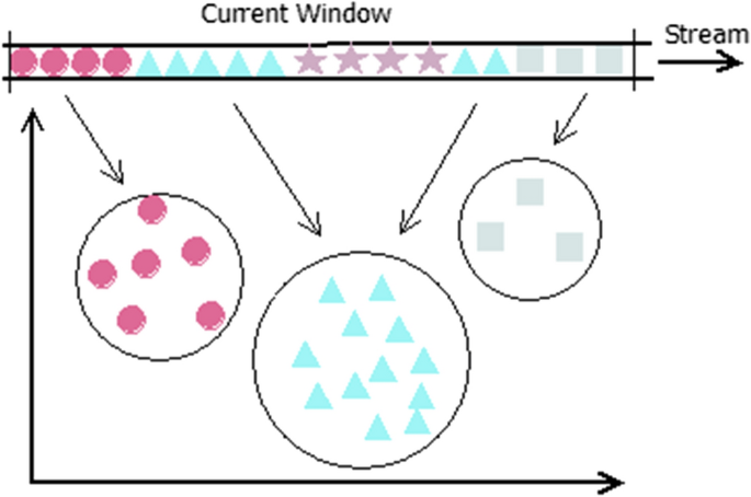

  

  Match_percentage denotes the number of samples in the current window that fit the selected clustering

• 2. The number of clusters in the selected clustering that do not include even a single sample from the current window is found out. The ratio of this number to the total number of clusters in the clustering is computed. This measure is termed as empty_cluster_count. Figure 4 shows the computation of empty_cluster_count.

  Fig. 4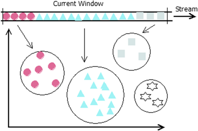

  

  The clusters that do not include even a single sample from the current window are counted for empty_cluster_count

• 3. The extent to which individual clusters match in terms of centre and radius. For each cluster in the selected clustering, the samples in the current window, which are included in that cluster, are taken. These samples are assumed to form a cluster, and then the mean (centre of the cluster) and the radius of this new cluster is calculated. In Fig. 5, the red coloured circle denotes this new cluster. The error in mean and the error in radius with the original cluster are measured. A detail on computing these errors is given in Algorithm 3. The errors are averaged over the total number of clusters contributing to the error in the particular clustering. This error computation will help to assess the match in size and location of the individual clusters.

  Fig. 5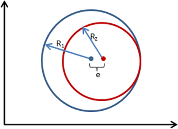

  

  Measures used to compute the error_in_mean and error_in_radius. 'e' denotes the error in mean and R2/R1 is the ratio of radii

Only those clusterings that cross a threshold value for the match_percentage are considered further in finding the matching candidate. The model with the highest match_percentage and the lowest total error is considered as the most matching model. The three error measures—empty_cluster_count, error_in_mean and error_in_radius contribute to the total error. The threshold value for the match_percentage is assumed to be user given. Depending on the specific domain, and dataset, this value can be decided by the user. More details on the computation of various measures can be seen in the algorithms, which are discussed in the next section.

The learning process

The learning process depends on the concept drift handling mechanism used. Hence the algorithm has two versions—one with fixed size window (Algorithm 1) and the other with explicit drift detection (Algorithm 2). In both, match finding from the repository happens in the same way (Algorithm 3). With window-based learning, samples in the current window are used to train the new model whereas, in explicit drift detection based learning, samples in the buffer are used to train the new model.

The initial model is created in an offline way, and this model is used to initialize the repository. On receiving each sample from the stream, the online component of the streaming algorithm works to create/update the summary statistics. When the window limit is reached, the offline part of stream learning algorithm has to be invoked. As shown in line 11 of Algorithm 1 (Fig. 6), this invocation only happens if there is no matching model in the repository. Otherwise, the matching model is retrieved from the repository, set as the current, active model, and the process continues by taking the next record from the stream, as shown in lines 8 and 9. If the new model gets created, it has to be added to the repository.

Fig. 6

Algorithm 1—Learning process with fixed-size window model

In explicit drift detection (Fig. 7), the drift parameters like warning threshold ${\uplambda }_{\mathrm{W}}$, alarm threshold ${\uplambda }_{\mathrm{A}}$ and the tolerance level δ have to be set (line 2 of Algorithm 2). The value of these parameters is determined dynamically from the current clustering, as it is discussed in [3]. On receiving each sample from the stream, tests against the warning threshold and alarm threshold have to be conducted. Also, threshold values and delta have to be updated each time a new model is set as the active model.

Fig. 7

Algorithm 2—The learning process with explicit drift detection

Samples from the current window/buffer are applied to each model in the repository to find the matching one. The match_percentage and the error measures described in the above section are computed. This procedure is explained in Algorithm 3 (Fig. 8).

Fig. 8

Algorithm 3—FindtheMatchingModel(S,M)

Memory requirements

A memory requirement analysis has been performed, considering CluStream as the base stream clustering algorithm. In CluStream, the micro-clusters saved in the on-line phase of the algorithm are treated as single points and are re-clustered to generate the macro-clusters [2]. The maximum value for k, the number of macro-clusters, is set to $\sqrt{N}$ by the algorithm which dynamically estimates k. Here N is the total number of points to be clustered and hence equal to the number of micro-clusters considered for macro-clustering. In CluStream algorithm, there is a user-defined limit on the maximum number of micro-clusters that can be maintained on-line by the system at any particular point of time. Suppose this limit is denoted by q. The algorithm also ensures this as the maximum number of micro-clusters from which macro-clustering is performed. Thus the upper bound on the number of macro-clusters created in a single clustering step can be estimated as $\sqrt{q}$. As mentioned before, a single cluster takes the size of (2d + 1) elements in the repository where d is the dimension of the dataset. So, after processing n number of windows or concept drift points, maximum $(n*\sqrt{q}*(2d+1))$ elements are required to store all the models in the repository. Usually, the nature of the dataset and the availability of primary memory decide the value of q. d is also a constant as far as the particular dataset is concerned. Hence the memory requirement of the model repository has a linear relationship to the number of windows/concept drift points processed till that time.

In addition to this storage required in secondary memory, CluStream has an inherent requirement of storing snapshots of micro-clusters periodically to secondary storage. At any point of time T, the maximum number of snapshots saved in memory will be $\left({\propto }^{l}+1\right).{log}_{\propto }T$ where $\propto$ is an integer ≥ 1 and $l$ is an integer > 1, as discussed in [2]. (2d + 3) elements are required to store a micro-cluster. Each snapshot can contain a maximum of q number of micro-clusters. Hence the total storage required for all the snapshots will be$\left({\propto }^{l}+1\right).{log}_{\propto }T*q*(2d+3)$. Since $\propto$, $l$ and $d$ are constants for a particular dataset, the storage requirement of snapshots is O(logT).

When cluster feature vector is used to represent clusters, the storage requirement is linearly related to the dimensionality of the stream. This relation holds good both in cases of snapshot storage and the model repository. Depending on the summary data structure used to store the clusters, the space requirements will vary.

Experiments

Experiments are conducted to validate the efficiency of the proposed algorithm on tracking concept recurrence in data stream clustering. Two experiment settings are developed with the following objectives.

• Experiment 1: Test the performance of the proposed method when window-based learning is used to manage the drift.

• Experiment 2: Assess the performance when explicit drift detection is used.

Experiments are conducted on a 2.4 GHz machine (2 processors) having 128 GB RAM, running Windows 10 Pro edition. Java is used to implement the algorithms. The experiments are based on heuristic approaches, and an optimal value is chosen for each dataset.

Since we are dealing with unsupervised learning, a suitable measure has to be adopted to evaluate the performance of this recurrence handling algorithm. As the concept in stream clustering is nothing but the data distribution itself, a measure to calculate the similarity between data distributions is chosen to show the effectiveness of the algorithm. It calculates the similarity in distribution between the current window and each previous window. Hellinger distance is taken as the measure to find this similarity in data distribution between windows. It has been checked if the model chosen from the repository, by the proposed algorithm corresponds to the least value of Hellinger distance among the previous windows.

Hellinger distance

An incremental way of computing the Hellinger distance is chosen to make it easy and suitable for data stream learning. As discussed in [8, 30], a histogram-based approach is adopted. The number of bins in a histogram is $\lfloor \sqrt{N}\rfloor$, where N is the total number of instances in each window. The histogram is created for each attribute separately, and distance is averaged to get the final Hellinger distance. At time point t, Hellinger distance between two distributions P and Q is calculated as

$${\delta }_{H}\left(t\right)= \frac{1}{d}\sum_{k=1}^{d}\sqrt{\sum_{i=1}^{b}{\left(\sqrt{\frac{{P}_{i,k}}{\sum_{j=1}^{b}{P}_{j,k}}}-\sqrt{\frac{{Q}_{i,k}}{\sum_{j=1}^{b}{Q}_{j,k}}}\right)}^{2}}$$

where d is the dimension of data, ${P}_{i,k}$ (or ${Q}_{i,k}$) is the count in bin i of histogram P (or Q) corresponding to the attribute k.

Datasets

Two real-world datasets, one synthetic dataset and two application datasets have been selected for conducting the experiments. The proposed methods are validated on these datasets.

The first real-world dataset used in our experiments is KDD-CUP'99 intrusion detection dataset. The 10% version of this dataset is used since it is more concentrated than the original one [20]. It has 494,020 records, with 34 continuous attributes. The intrusions are classified into 22 different types, hence forming a total of 23 classes, including the normal connection. Min–max normalization is applied to the data to prepare it for experiments [6]. The second real dataset is the Localization Data for Person Activity from UCI machine learning repository. It has 164,860 instances with three numeric attributes and 11 classes.

The synthetic dataset is generated using Random RBF generator available in Massive Online Analysis (MOA) software. Two streams are generated from Random RBF generator by varying the parameters like the number of centroids and the number of classes. These streams are then combined to create the effect of concept recurrence. Chunks of 10,000 records from each stream are placed in alternate order to create the final stream.

Results and discussion

The following subsections discuss the results of the two set of experiments conducted—window-based learning and explicit drift detection.

Window-based learning

Determining the size of the window is an important concern in window-based learning [10, 37]. We have tried the window sizes 1000, 2000 and 5000 in our experiments with real and synthetic datasets. The results shown in this section corresponds to window size 5000; Person Activity dataset is an exception, for which it is 1000. A discussion on selecting the window size is included in the sub-section “Choosing parameter values”. The match_threshold is set to 99%.

KDD-CUP'99 intrusion detection dataset

The occurrence of intrusion types in KDD-CUP dataset is shown in Fig. 9. The intrusion classes are numbered 1 to 22 by keeping the same order as they are listed in dataset description of KDD-CUP'99 dataset¹. Class 23 refers to the normal connection. This dataset has been a favourite choice for validating data stream classification and clustering algorithms, due to its highly evolving nature [2]. The frequent appearance and disappearance of new classes, significant evolution over time, highly imbalanced classes are the characteristics that make this dataset quite challenging. This dataset undergoes both concept drift and concept evolution [22]. Moreover, we can see the virtual concept drift in this dataset [19]. Smurf (class label 18) and Neptune (class label 10) classes form the majority of attacks as it can be observed in Fig. 9.

Fig. 9

Class labels in KDD-CUP'99 intrusion detection dataset

Figure 10, a pictorial representation of the information included in Table 1, illustrates the concept recurrence identified in KDD-CUP dataset. Time of the creation of reused models is shown on the y-axis. For each model represented on y-axis, the circles lying on the corresponding line indicate the time-points when that model is reused. The reuse of each model is shown in a different colour. For example, the circles in red colour denote the reuse of the model created at time-point 0.5 × 10⁵. It has been reused many times after 1.6 × 10⁵, when the same concept recurs. Similarly, the other reused models are also included in the figure.

Fig. 10

Concept recurrence and model reuse in KDD-Cup'99 intrusion detection dataset

Table 1 Model reuse in KDD-CUP'99 intrusion detection dataset

From Figs. 9 and 10, it is evident that the model reuse happens mostly when the same attack type repeats. The class labels 10 (attack type neptune) and 18 (attack type smurf) continue for relatively long duration in this dataset. Figure 10 shows that the models created for these classes are reused several times when the same class recurs. It is observed that the same clustering structure survives as long as the category of attack is the same, which is a known property of KDD-CUP'99 intrusion detection dataset, as it is discussed in [38]. Thus it supports the fact that the proposed algorithm is successful in identifying the recurring concepts.

Hellinger distance is computed to cross-check the correctness of the algorithm further. For each window, its Hellinger distance to all the previous windows is calculated. It is checked if the most similar distribution identified in terms of Hellinger distance and the most matching model selected by the proposed algorithm refer to the same window in history. The proposed algorithm effectively computed the match to each previous model in the repository, and the computed Hellinger distances agreed with these match values. From this dataset, two windows, which are identified to be of recurring concept, are chosen as examples to show the results—the window at 4.4 × 10⁵ from smurf class and the window at 3.8 × 10⁵ from neptune class.

The Hellinger distances calculated for the window 4.4 × 10⁵ to each of its previous windows is shown in Fig. 11. As shown in Table 1, the algorithm identified the model created at 0.5 × 10⁵ to be the most matching model for this window. i.e., the concept at window 0.5 × 10⁵ recurs at 4.4 × 10⁵. From Fig. 11, it is evident that among the Hellinger distances computed for the window 4.4 × 10⁵, the one calculated for 0.5 × 10⁵ is the minimum. It is highlighted using a blue circle in the figure. Thus it proves that the algorithm correctly identified the most matching model from the repository. Similar results can be found in Fig. 12 for the window 3.8 × 10⁵.

Fig. 11

Hellinger distances for the window 4.4 × 10⁵ of KDD-CUP dataset

Fig. 12

Hellinger distances calculated for the window 3.8 × 10⁵ KDD-CUP’99 dataset

Person Activity dataset

As it can be observed in Fig. 13, the class labels or the person activities change very frequently in Person Activity dataset. The data distribution also changes rapidly, leading to fast concept changes. A window size of 5000 is too big to capture these concept changes. Hence we got better results for the window size 1000. Figure 14 shows the model reuse in Person Activity dataset. Time of the creation of reused models is shown on y-axis of the figure.

Fig. 13

The class labels in Person Activity dataset

Fig. 14

Concept recurrence and Model reuse in Person Activity dataset

Hellinger distance based analysis is shown in Fig. 15. Among the recurring concepts shown in Fig. 14, the window 12.6 × 10⁴ is chosen as an example, and its distance to its previous windows is shown in Fig. 15. As seen in the figure, Hellinger distance is the least for window 12.4 × 10⁴. The proposed algorithm also has chosen the model created at 12.4 × 10⁴ as the most matching model for the concept at 12.6 × 10⁴.

Fig. 15

Hellinger distance for the window 12.6 × 10⁴ in Person Activity dataset

Synthetic dataset

Figure 16 shows the class labels in the synthetic dataset. There are two classes—class 0 and class 1. The classes are made recurring to check the performance of the algorithm. Since the match_threshold is set to 99%, only one class meets the model reuse requirements set by the proposed algorithm. The model created for class 0 is reused when the same class repeats. As it can be observed in Fig. 17, the model created at time point 1 × 10⁴ is reused at 2.5 × 10⁴, 4.5 × 10⁴ and 6.5 × 10⁴.

Fig. 16

Class labels in the synthetic dataset

Fig. 17

Concept recurrence and the model reuse in the synthetic dataset

Figure 18 shows the Hellinger distance of the window at 6.5 × 10⁴ to its previous windows. It has a minimum distance to the window at 1 × 10⁴ (highlighted using the blue circle in the figure).

Fig. 18

Hellinger distance of window 6.5 × 10⁴ to all the previous windows

Learning with explicit drift detection

The alarm threshold λ_A, warning threshold λ_w, and the tolerance level δ are the important parameters to be set while using the Page-Hinkley test. This section includes the results of applying Algorithm 2 to the real and synthetic datasets. λ_A is set to be the average cluster radius of the active model, λ_w is $\frac{{\lambda }_{A}}{3}$ and δ is ${\lambda }_{A}*0.1$. The match_threshold is set to be 99%. A parameter significance test is conducted to understand the influence of the test parameters, and the observations are included in the sub-section “Choosing parameter values”.

KDD-CUP’99 intrusion detection dataset

Figure 19 shows the concept drift points in KDD-CUP dataset. The vertical dashed lines represent the concept drift points identified by the Page-Hinkley test. Intra-class drift is very rare in this dataset as we can observe in the figure. When neptune and smurf attack types persist for a long duration, there is hardly any concept drift identified within those classes. Once a drift is detected, the repository is searched for finding a matching model.

Fig. 19

Class labels and the concept drift points in KDD-CUP dataset

Figure 20 shows the model reuse in this dataset when explicit drift detection is employed. Time of creation of the reused models is shown on the y-axis, and reuse of different models is shown in different colours.

Fig. 20

Concept recurrence in KDD-CUP dataset with explicit drift detection

Person Activity dataset

The results of Person Activity dataset with explicit drift detection is shown in Fig. 21. As it can be seen in the figure, altogether there is more model reuses compared to the fixed size window based learning. The results on this dataset support the fact that explicit drift detection is better compared to window based learning in data streams with frequent concept drifts. Explicit drift detection makes it possible that the models are developed for specific concepts. Unlike the other variant, there is no need to unnecessarily generalize the model to include a fixed number of samples from the stream. Person Activity dataset has frequent concept changes, and the fixed size window-based method is insufficient to learn these changes on time. While explicit drift detection is employed, drifts are identified on the right time and models are created or reused accordingly. Hence we get more model reuse here.

Fig. 21

Model reuse in Person Activity dataset while drifts are detected explicitly

Synthetic dataset

Figure 22 shows the model reuses in the synthetic dataset. Even minute concept drifts are captured in this dataset when we set the alarm threshold to the average cluster radius of the active model. But the model reuse happens only with class 0, as it is evident from the figure. Even though there are concept drifts in class 1, the model reuse requirements are not met, and hence the model reuse is hardly possible with this class.

Fig. 22

Model reuse in the synthetic dataset with explicit drift detection

From the experiments, we observed that the proposed algorithm could identify the recurring concepts in data stream clustering scenarios. It finds out the most similar data distribution from the history if one exists, and reuses the corresponding model instead of building a new model from scratch. At the same time, the experiments show that the algorithm might fail if the concept changes are frequent. If the data distributions change very rapidly, the algorithm does not get enough time to learn the concept and store it as a model in the repository. Otherwise, if the concepts are fairly stable, their re-occurrence is captured by the algorithm. The Hellinger distance based analysis also supports this observation.

Application datasets

Concept recurrence is a common scenario in many real-world applications. When concepts are related to hidden contexts, re-appearance of contexts leads to concept recurrence. The changes in season, economic conditions, fashion etc. are examples of contexts that drive related concepts in real-world streams. Two such streams are selected for conducting experiments.

Weather data stream

Weather data from the Automatic Weather Station (AWS) of Advanced Centre for Atmospheric Radar Research (ACARR), Cochin University of Science and Technology, is used for this experiment. Data collected at 30-min interval contains three weather parameters—temperature, humidity and net radiation. The stream has approximately data of 3.5 years, starting from January 2016 onwards, making a total of 61,754 entries. As in the other experiments, data is min–max normalized. The off-line clustering is performed on the initial 5000 samples to create the first model.

Table 2 shows the concept recurrence and model reuse in this dataset when fixed-size window based learning is applied. The results shown correspond to a window size of 100—which represents approximately data of 2 consecutive days—and a match threshold of 95%. No match could be identified by the system when the match threshold was set to 99%. From the table, some concepts can be found recurring in a yearly manner when the same seasons repeat. For example, models created on 12/07/16, 29/04/18 and 07/05/18 can be found recurring next year when the same seasons reappear. Concept recurrences within a season can also be found in the table.

Table 2 Concept recurrence and model reuse in weather dataset

The Hellinger distances computed for the window at 57,000 (around 9/3/19) to its previous windows is shown in Fig. 23. As evident from this figure, there is a seasonal variation in Hellinger distance as well. The distance is less for the windows from the same season in the previous years. Figure 24 depicts the models for which the match_percentage crosses the match_threshold for the window 57,000. Eleven models (shown as blue dots in the figure) are found crossing the match_threshold, and all of them are from the same season of the previous year. The Hellinger distance based analysis in Fig. 23 also agrees with this result—i.e., matching models correspond to the low Hellinger distances as visible in the figure. The most matching model is picked up from these 11 matching models.

Fig. 23

Hellinger distances computed for the window at 57,000 (9/3/19)

Fig. 24

The models that cross the match threshold for window 57,000

The weather dataset is used in experiments of explicit drift detection as well. Even though many concept drift points are identified in the stream, concept recurrences are rarely found. Concept learned at 58,930 (5/5/19) is identified to be matching to five models learned in the past, with the most matching one being the model at 45,994 (19/6/18).

Stock time series data

A stock time-series data available in Kaggle datasets is also used in the experiments. DJIA 30 stock time-series data [33] contains daily stock price data of 29 companies for 12 years (2006 to 2018), from which the first one named AABA is selected here. This dataset is relatively small compared to the other datasets used in our experiments. It has seven columns and 3020 entries in total. Out of the available seven columns, attributes named date, volume and name are removed, and the stream is simulated with the remaining four parameters. The used attributes include opening price, closing price, highest price and lowest price. Table 3 shows the concept recurrence when a window of size 100 is used.

Table 3 Concept recurrence and model reuse in the stock dataset

Since the data is a daily basis, a window size of 100 approximately refers to the quarter of a year. Thus the clustering over a window of samples indicates how the data was distributed in that quarter. Also, the recurrence check tries to find out the similarity between the distributions of data (based on the stock prices) in different quarters.

The last window among the observed concept recurrences—2800—is taken as an example, and its Hellinger distances to previous windows are shown in Fig. 25. The blue circle in the figure denotes the window with minimum Hellinger distance—2400—which is identified to be the most matching model by the system as well. While recurrence check using explicit drift detection is performed, the model created at 1133 is found reused at 1343 and 1749.

Fig. 25

Hellinger distance of the window 2800 to its previous windows for the stock time series dataset

Memory usage

The maximum memory requirement for storing models in the repository for each dataset is shown in Table 4. On memory analysis, it is found that a maximum of $(n*\sqrt{q}*(2d+1))$ elements are required for each dataset where n is the number of windows/concept drift points identified in the stream. For the first three datasets, the value of q is set to 100; for the application datasets, as they are smaller in length, q is set to 20. In our experiments, the double data type of java is used to store each element of the cluster feature vector in memory. The memory requirement in KB, shown in Table 4 is calculated on the basis of this information.

Table 4 Maximum memory requirements for storing the models

The size of the repository required for storing the models is not even five percent of the total volume of the stream in all the cases. Providing this space in secondary storage is not a great deal as far as the current storage capabilities are concerned. The system can indeed run out of storage when the stream grows infinitely. Adopting suitable measures to remove the old unnecessary models from the repository is a need of the system. At the same time, it is evident that the cluster feature vector is an efficient way to store the models in memory.

Choosing parameter values

Fixed size window based learning is the most straightforward approach if the user has an idea about the time scale of the change [15]. Large windows are suitable for streams with fairly long, stable concepts, whereas they prove less accurate for streams with frequent concept drifts. Small windows are ideal in case of frequent changes. As mentioned earlier, we have conducted experiments with windows of size 1000, 2000 and 5000 for real and synthetic streams. Since the KDD-CUP and the synthetic stream have stable concepts that endure for a long time, all these window sizes produced good results.

In Person Activity dataset, it is observed that the data distribution changes very frequently and hence large window sizes produce models, too much generalized to fit the whole window. The small changes happened within the window are not captured. For this reason, the window size of 1000 produced better results on this dataset. In case of application datasets, a reasonable size was chosen based on the characteristics of the domain. For weather data, a window included the data of a few days, and for stock price data it included data of a quarter. Optimum window size has to be chosen depending on the characteristics of the data as it is discussed in the survey [15].

In explicit drift detection based learning, the threshold values (λ_A and λ_w), and the tolerance level δ are the parameters to be chosen by the user. They are made partially self-adjustable depending on the average radius of the active clustering. Result of the parameter sensitivity analysis conducted on KDD-CUP dataset with λ_A = {1, 1.5, 2} times the average cluster radius and δ = {0.1, 0.01} times λ_A is shown in Table 5. In this dataset, the data distribution is known to be associated with the class label. Hence it is possible to verify the false alarms, detection delay and missed detections. The minimum buffer size is set to 500 to ensure the quality of the clustering. Hence class occurrences with less than 500 samples are discarded from this analysis. The normal class is known to be containing intra-class concept drifts, which are also not considered.

Table 5 Parameter sensitivity analysis with KDD-CUP dataset

As it can be observed in Table 5, an increase in λ_A reduces the false alarm ratio but causes more missed detections. The smaller value of δ reduces the detection delay at the cost of increased false alarm ratio. Hence these parameters have to be fixed depending on the tolerable limit of missed detection, false alarm ratio and detection delay. This acceptable limit is user’s choice or domain-dependent. From the results, λ_A = 1 * average cluster radius and δ = 0.1 * λ_A looks better as it has zero missed detections, very less false alarm ratio and tolerable detection delay compared to others. So, we have selected these values in our experiments.

Change in the base clustering algorithm

Table 6 shows the concept recurrence detected in KDD-Cup'99 intrusion detection dataset with StreamKM++ [1] algorithm in the base layer. StreamKM++ is an algorithm that uses the coreset tree as the data structure to store the summary of the stream. As expected with KDD-CUP dataset, the concept recurrence happens when the same attack repeats. A clustering structure generated for a class survives till the end of that class except for the normal connection. Even with a change in the base clustering algorithm, the results are comparable.

Table 6 Model reuse in KDD-CUP dataset with StreamKM++ algorithm

In the current form, the proposed method works only with object-based clustering algorithms producing hyper-sphere shaped clusters. The attribute-based clustering algorithms or arbitrary shaped clusters cannot be directly used in the current settings. The reason is that the method of finding the similarity between the points and a clustering structure will not work as expected with attribute-based algorithms or arbitrary-shaped clusters. It can also be noted that a change in the summary data structure does not affect the results.

Conclusions

Concept recurrence is an interesting phenomenon in data stream mining. Research happened so far on tracking and prediction of recurring concepts has mainly focused on classification problems. This paper presents an algorithm for tracking concepts and identifying concept recurrence in data stream clustering. Based on the literature survey conducted, this is the first algorithm addressing the problem of concept recurrence in stream clustering. It proposes a novel method of identifying concept equivalence by checking the similarity in clustering structures. The concept comparison is made possible with minimal storage, as it is the essential requirement of a data stream mining system.

Two different dimensions of concept drift detection have been addressed in the experiments; the widely accepted method of fixed size windows and the explicit identification of drift using a statistical test. It is found that the former is the simplest and effective approach in case of long stable concepts or if the time scale of change is known. The results supported the fact that even though explicit drift detection incurs the extra cost of identifying the drift, it proves more efficient in dynamic scenarios. Explicit drift detection helps the window size to be variable to fit the length of the concept. Experiment with the Person Activity dataset supports this observation. Hellinger distance based analysis is used to verify the correctness of the algorithm. Experiments conducted on different datasets illustrate that the algorithm is capable of finding the most matching model from the repository.

As future work, we plan to study the pattern in recurrence and anticipation of concept drift in data stream clustering. Also, the utilization of context information to avoid checking all the models in the repository is part of the future plan.

References

Ackermann MR, Lammersen C, Sohler C, Swierkot K, Raupach C. StreamKM++: a clustering algorithm for data streams. J Exp Algorithmics. 2012;17:173–87. https://doi.org/10.1145/2133803.2184450.
Aggarwal CC, Watson TJ, Ctr R, Han J, Wang J, Yu PS. A framework for clustering evolving data streams. In: Proceedings of the 29th international conference on very large data bases. 2003. pp. 81–92. https://doi.org/10.1016/B978-012722442-8/50016-1
De Andrade Silva J, Hruschka ER, Gama J. An evolutionary algorithm for clustering data streams with a variable number of clusters. Expert Syst Appl. 2017;67:228–38. https://doi.org/10.1016/j.eswa.2016.09.020.
Barbará D. Requirements for clustering data streams. ACM SIGKDD Explor Newsl. 2002;3(2):23. https://doi.org/10.1145/507515.507519.
Cao F, Ester M, Qian W, Zhou A. Density-based clustering over an evolving data stream with noise. In: SDM. 2006. pp. 326–37. https://doi.org/10.1145/1552303.1552307.
Chen Y, Tu L. Density-based clustering for real-time stream data. In: Proceedings of the 13th ACM SIGKDD international conference on knowledge discovery and data mining—KDD ’07. 2007;133. https://doi.org/10.1145/1281192.1281210
De Andrade Silva J, Hruschka ER. Extending k-means-based algorithms for evolving data streams with variable number of clusters. In: Proceedings—10th international conference on machine learning and applications, ICMLA 2011. 2011;2:14–19. https://doi.org/10.1109/ICMLA.2011.67.
Ditzler G, Polikar R. Hellinger distance based drift detection for nonstationary environments. In: IEEE symposium on computational intelligence in dynamic and uncertain environments. 2011. pp. 41–8. https://doi.org/10.1109/CIDUE.2011.5948491.
Faria ER, Uberlândia SC, Barros RC, Carlos S, Carvalho ACPLF, Carlos S. Improving the offline clustering stage of data stream algorithms in scenarios with variable number of clusters. 2012;829–30.
Gama JA. A survey on concept drift adaptation. ACM Comput Surv. 2014;46(44):1–37. https://doi.org/10.1145/2523813.
Gama J, Kosina P. Learning about the learning process. In: Proc. of the 10th int. conf. on advances in intelligent data analysis. 2011. pp. 162–72. https://doi.org/10.1007/978-3-642-24800-9_17
Gomes JB, Menasalvas E, Sousa PAC. Learning recurring concepts from data streams with a context-aware ensemble. In: Proceedings of the ACM symposium on applied computing (SAC’11). 2011. pp. 994–9. https://doi.org/10.1145/1982185.1982403.
Gomes JB, Sousa PAC, Menasalvas E. Tracking recurrent concepts using context. Intell Data Anal. 2012;16:803–25. https://doi.org/10.3233/IDA-2012-0552.
Guha S, Mishra N, Motwani R, O'Callaghan L. Clustering data streams. In: Proceedings 41st annual symposium on foundations of computer science, Redondo Beach, CA, USA, 2000, pp. 359–66. https://doi.org/10.1109/SFCS.2000.892124.
Iwashita AS. An overview on concept drift learning. IEEE Access. 2019;7(Section III):1532–47. https://doi.org/10.1109/ACCESS.2018.2886026.
Katakis I, Tsoumakas G, Vlahavas I. Tracking recurring contexts using ensemble classifiers: an application to email filtering. Knowl Inf Syst. 2010;22(3):371–91. https://doi.org/10.1007/s10115-009-0206-2.
Kifer D, Ben-david S, Gehrke J. Detecting change in data streams. In: Proceedings of the 30th VLDB conference. 2004. pp. 180–91.
Kubat M. Second tier for decision trees. In: ICML'96: proceedings of the thirteenth international conference on international conference on machine learning. 1996. pp. 293–301.
Li P, Wu X, Hu X, Wang H. Learning concept-drifting data streams with random ensemble decision trees. Neurocomputing. 2015;166:68–83. https://doi.org/10.1016/j.neucom.2015.04.024.
Masud M, Gao J, Khan L, Han J, Thuraisingham BM. Classification and novel class detection in concept-drifting data streams under time constraints. IEEE Trans Knowl Data Eng. 2011;23(6):859–74. https://doi.org/10.1109/TKDE.2010.61.
Miguel Ángel A, João Bártolo G, Ernestina M. Predicting recurring concepts on data-streams by means of a meta-model and a fuzzy similarity function. Expert Syst Appl. 2016;46:87–105. https://doi.org/10.1016/j.eswa.2015.10.022.
Mohamad S, Sayed-mouchaweh M, Bouchachia A. Active learning for classifying data streams with unknown number of classes. Neural Netw. 2017;98:1–15. https://doi.org/10.1016/J.NEUNET.2017.10.004.
Naldi MC, Fontana A, Campello RJGB. Comparison among methods for k estimation in k-means. In: ISDA 2009—9th international conference on intelligent systems design and applications. 2009. pp. 1006–13. https://doi.org/10.1109/ISDA.2009.78.
Namitha K, Santhosh G. Concept drift detection in data stream clustering and its application on weather data. Int J Agric Environ Inf Syst. 2020;11:67–85. https://doi.org/10.4018/IJAEIS.2020010104.
Paulo B. Learning recurring concepts from data streams in ubiquitous environments. Philosophy. 2011; September.
Rodrigues PP, Gama J, Pedroso JP. ODAC: hierarchical clustering of time series data streams. IEEE Trans Knowl Data Eng. 2008;20(5):615–27. https://doi.org/10.1109/TKDE.2007.190727.
Rousseeuw PJ. Silhouettes: a graphical aid to the interpretation and validation of cluster analysis. J Comput Appl Math. 1987;20:53–65. https://doi.org/10.1016/0377-0427(87)90125-7.
Sakamoto Y, Fukui KI, Gama J, Nicklas D, Moriyama K, Numao M. Concept drift detection with clustering via statistical change detection methods. In: Proceedings—2015 IEEE international conference on knowledge and systems engineering, KSE. 2015. pp. 37–42. https://doi.org/10.1109/KSE.2015.19.
Serakiotou N. Change detection. Stanford Exploration Project. 1987.
Sethi TS, Kantardzic M. On the reliable detection of concept drift from streaming unlabeled data. Expert Syst Appl. 2017;82:77–99. https://doi.org/10.1016/j.eswa.2017.04.008.
Silva JA, Faria ER, Barros RC, Hruschka ER, De Carvalho ACPLF, Gama J. Data stream clustering. ACM Comput Surv. 2013;46(1):1–31. https://doi.org/10.1145/2522968.2522981.
Song G, Ye Y, Zhang H, Xu X, Lau R, Liu F. Dynamic clustering forest: an ensemble framework to efficiently classify textual data stream with concept drift. Inf Sci. 2016;357:125–43. https://doi.org/10.1016/j.ins.2016.03.043.
szrlee DJIA 30 Stock Time Series. 2018. www.kaggle.com/szrlee/stock-time-series-20050101-to-20171231. Accessed 03 Oct 2019.
Vendramin L, Jaskowiak PA, Campello RJGB. On the combination of relative clustering validity criteria. In: Proceedings of the 25th international conference on scientific and statistical database management—SSDBM. 2013;1. https://doi.org/10.1145/2484838.2484844
Webb GI, Hyde R, Cao H, Nguyen HL, Petitjean F. Characterizing concept drift. Data Min Knowl Discov. 2016;30(4):964–94. https://doi.org/10.1007/s10618-015-0448-4.
Widmer G. Tracking context changes through meta-learning. Mach Learn. 1997;27(3):259–86. https://doi.org/10.1023/A:1007365809034.
Widmer G, Kubat M. Learning in the presence of concept drift and hidden contexts. Mach Learn. 1996;23(1):69–101. https://doi.org/10.1007/BF00116900.
Yang Y, Wu X, Zhu X. Mining in anticipation for concept change: proactive-reactive prediction in data streams. Data Min Knowl Discov. 2006;13(3):261–89. https://doi.org/10.1007/s10618-006-0050-x.
Zhang T, Ramakrishnan R, Livny M. BIRCH: an efficient data clustering databases method for very large. In: ACM SIGMOD international conference on management of data. 1996;1:103–114. https://doi.org/10.1145/233269.233324.
Zhang X, Germain C, Sebag M. Adaptively detecting changes in autonomic grid computing. In: Proceedings—IEEE/ACM international workshop on grid computing, 2010. pp. 387–92. https://doi.org/10.1109/GRID.2010.5698017.
Acknowledgements
The authors thank both the funding agencies; UGC for granting RUSA scheme and DST for awarding PURSE scheme; which were utilized to build the infrastructure needed for this research. The authors also thank the technical staff and faculty at ACARR (Advanced Centre for Atmospheric Radar Research), Cochin University of Science and Technology for supporting this work.
Funding
The authors thank both the funding agencies; UGC for granting RUSA scheme and DST for awarding PURSE scheme; which were utilized to build the infrastructure needed for this research.
Author information
Authors and Affiliations
Contributions
NK designed and implemented the algorithms for tracking concept recurrence in data stream clustering. NK collected the datasets and conducted the experiments for validating the algorithms. SK supervised the design and implementation of algorithms. Both the authors were involved in writing the manuscript. Both authors read and approved the final manuscript.
Corresponding author
Ethics declarations
Competing interests
The authors declare that they have no competing interests.
Additional information
Publisher's Note
Springer Nature remains neutral with regard to jurisdictional claims in published maps and institutional affiliations.
Rights and permissions
Open Access This article is licensed under a Creative Commons Attribution 4.0 International License, which permits use, sharing, adaptation, distribution and reproduction in any medium or format, as long as you give appropriate credit to the original author(s) and the source, provide a link to the Creative Commons licence, and indicate if changes were made. The images or other third party material in this article are included in the article's Creative Commons licence, unless indicated otherwise in a credit line to the material. If material is not included in the article's Creative Commons licence and your intended use is not permitted by statutory regulation or exceeds the permitted use, you will need to obtain permission directly from the copyright holder. To view a copy of this licence, visit http://creativecommons.org/licenses/by/4.0/.
About this article
Cite this article
Namitha, K., Santhosh Kumar, G. Learning in the presence of concept recurrence in data stream clustering. J Big Data 7, 75 (2020). https://doi.org/10.1186/s40537-020-00354-1
Received:
Accepted:
Published:
DOI: https://doi.org/10.1186/s40537-020-00354-1