Analyzing MRI scans to detect glioblastoma tumor using hybrid deep belief networks

Abstract

Glioblastoma (GBM) is a stage 4 malignant tumor in which a large portion of tumor cells are reproducing and dividing at any moment. These tumors are life threatening and may result in partial or complete mental and physical disability. In this study, we have proposed a classification model using hybrid deep belief networks (DBN) to classify magnetic resonance imaging (MRI) for GBM tumor. DBN is composed of stacked restricted Boltzmann machines (RBM). DBN often requires a large number of hidden layers that consists of large number of neurons to learn the best features from the raw image data. Hence, computational and space complexity is high and requires a lot of training time. The proposed approach combines DTW with DBN to improve the efficiency of existing DBN model. The results are validated using several statistical parameters. Statistical validation verifies that the combination of DTW and DBN outperformed the other classifiers in terms of training time, space complexity and classification accuracy.

Introduction

Glioblastoma (GBM) is a stage IV aggressive malignant brain tumor, which is generally found in the cerebral hemispheres of the brain [1]. The treatment of GBM tumor is very difficult and cure is not possible in most of the cases. The treatment can only slow down the progress of the cancer and may reduce the symptoms and discomfort. The diagnosis of GBM contains neurological exams, imaging tests i.e. MRI and biopsy. The GBM tumor may occur at any age; however, the high majority of the patients are adults. The symptoms of GBM may include worse headache, nausea, vomiting and seizures (Fig. 1).

Fig. 1

Glioblastoma brain tumor

Medical science is equipped with advanced devices and technology. MRI machines are able to capture high contrast images of the brain and other parts of the body. These MRI scans are very useful to diagnose and detect tumors and other defected cells. However, sufficient knowledge and experience is desirable in order to read and understand these MRI scans. Sometimes, unavailability of such trained people may delay the diagnosis process. Therefore, in order to automate the process, a classification model can be developed using machine learning methods. Artificial neural network (ANN) is one of the powerful approaches in machine learning which are able to handle large amounts of data with desirable accuracy. Advancement in ANN came up with deep neural architectures i.e. convolutional neural network (CNN) and recurrent neural network (RNN). Deep neural network [2] allows us to understand the hidden patterns from the complex data and images. Deep belief networks (DBN) is a class of deep neural networks with multiple layers of hidden units in which connections are established between layers rather than units within each layer. Each layer in DBN is a restricted Boltzmann machine (RBM) stacked against each other to construct the DBN. Deep learning approaches are able to automatically extract the features from the large data sets, however the correctness of the extracted features are not guaranteed [3,4,5]. In order to overcome this issue, this article proposed a DTW based DBN approach for image classification.

The rest of the article is organized as follows: In “Literature review section”, state of art literature review is presented. “Materials and methods” section discusses the materials and methods that consist of the description of the data set and methodology used in the study. “Results and discussion” section presents results and discussion and “Conclusion and future scope” section concludes the article with limitation and future scope of the article.

Literature review

Deep learning approaches have gained a lot of attention in the last decade in the medical domain. Deep learning methods are capable of extracting complex features from the raw data and able to construct new features from the existing one. Affonso et al. [6] argued that human inspection is a time consuming process in several industries to check the quality of materials. Automatization could improve this process through digital image processing. However, accuracy and computational cost are very important and therefore there should be a balance between the two. The authors used convolutional neural networks (CNN) with feature descriptors to analyze real world data of woods samples from industries. They concluded that CNN along with the feature descriptor provides a better accuracy in classification of the image data. Qayyum et al. [7] proposed a CNN based approach for content-based image retrieval system for medical image classification. They used a rich data set of medical images with twenty-four classes for analysis. They proposed that learning discriminative features directly from the images may reduce the semantic gaps and would improve the classification. They achieved a classification accuracy of 99.77% with deep CNN.

Jaiswal et al. [2], used CNN to classify the pneumonia using chest X-ray. They used publically available chest x-ray dataset from RSNA (Radiological Society of North America). They evaluated several deep learning models and found that Mask-RNN is able to achieve better accuracy among others. In [8], Litjen et al. conducted a comprehensive state of art survey on various methods, applications of deep learning approaches in medical image analysis, segmentation and object detection. They illustrated how deep learning is facilitating several aspects of the medical domain. Khatami et al. [3] proposed an image classification approach for radiography images. They applied Kolmogorov–Smirnov test to find the most discriminative features from the radiography images. They argue that DTW can slightly improve the classification performance using deep networks. Another study [9] extended the deep convolutional neural network to classify the echocardiography video images to assist in the diagnosis of heart disease. Data-driven learning frameworks by incorporating both spatial and temporal information from video images have been given as input to the CNN in this study and they have achieved 92.1% accuracy. They also mentioned that incorporating feature extraction helps to improve the classification performance of deep neural networks. Gao et al. [5] proposed a deep learning based model to diagnose Alzheimer disease using CT scans of the brain. They mentioned that CNN provides desirable accuracy that helps in early diagnosis of Alzheimer disease. They developed an advanced CNN incorporating both 2D and 3D CNN networks. The stated that the modified CNN was able to achieve better accuracy and classification in comparison to other 2D CNN models. Sharma et al. [10] used a deep learning framework to diagnose cancer cells. They developed a CNN model to classify the cancer image data and compared with other traditional approaches. They also found that CNN performs better than other methods. Al-Rahhal et al. [11] developed a deep learning framework to classify the electrocardiogram signals (ECG) to detect the heart disease. The extracted suitable features from the ECG data using stacked auto-encoders. Next, a softmax regression layer is added on the top of the hidden layers in the deep neural network. Moreover, expert recommendations are considered to label the ECG signals. They mentioned that the proposed approach achieved better accuracy than other state of the art approaches.

In another study [12], Tang et al. used multi-scale representation to capture and represent features from the medical images. Further, extracted features were encoded using Fisher vector technique. The authors claimed that the proposed approach demonstrated a superior performance on the data set. Zhong et al. [13] stated that the deep learning model specifically CNN needs a sufficiently large number of labeled samples to train the model. However, real world hyper spectral labeled images are limited in the amount. Therefore, deep learning may not be suitable for such kind of data. They suggested that DBN is able to deal with this issue as it provides unsupervised pre-training to the unlabeled samples but may result in several dead hidden units. They proposed an approach to deal with this problem and obtained better performance than the original DBN. Zhao et al. [14] proposed a feature learning method known as discriminant DBN for learning high-level features for image classification. These discriminant features are learned by ensemble learning mechanism with DBN in an unsupervised manner. Wang et al. [15] suggested a semi supervised DBN based on Boltzmann machine by introducing the relevant constraint and the supervised information are equivalently integrated into the learning process of this restricted Boltzmann machine and then, this model is constructed to improve the classification accuracy. Shi and Chi [16] proposed a hyper-spectral image classification method. This method has exploited the 3D spectral-spatial information using 3D deep neural networks. They constructed a super pixel to generate the spatial image to increase the spectral-spatial similarity and diversity. Next, a 3D super pixel based sample filling method has been applied to solve the misclassification issue and finally, a 3D recurrent CNN had been used for classification of images. Similarly, Paoletti et al. [17] proposed a deep CNN based image classification model for hyper-spectral images by presenting a 3D network based CNN that uses both spatial and spectral information. They have also implemented mirroring strategy to effectively process border areas in the images. The development of computational models for medical image diagnosis raised a new level of interventional treatment. Therefore, medical image processing is now one of the most effective ways to quickly diagnose the diseases and assist the medical staff in quick decision making. As a solution, machine learning techniques are being used to automate the diagnosis process since last decade. However, traditional machine learning methods are not sufficient to deal with complex problems. Therefore, deep learning methods are trying to resolve the limitations of machine learning based techniques. In this work, an attempt has been made to show a clear cut differentiation between deep learning based methods and non-deep learning based methods for image classification.

Materials and methods

Data set description

The dataset obtained from cancer imaging archive repository collections of Rider Neuro MRI images [18]. Rider Neuro MRI images consist of a data set of 19 patients with recurrent GBM. The 19 patients had repeat dynamic contrast-enhanced MRI (DCE-MRI) datasets on the same 1.5T imaging magnet. The total number of high contrast images is 70,220 for 19 patients. The total size of the data set was 7.3 Gigabytes. The image data contains two classes: images with the presence of GBM tumor and images without GBM. Figure 2 illustrates the two classes (with or without presence of GBM tumor) in the data set.

Fig. 2

a Represents a normal brain. b–h represents brain with GBM tumour

Proposed approach

In this study, a novel approach is proposed to classify the MRI images using a deep learning framework. Figure 3 illustrates the proposed framework for image classification in three stages. The first stage performs the data preprocessing that consists of feature extraction using DWT, vectorization and construction of additional features for processing. The second stage deals with dimensionality reduction of the images using principal component analysis (PCA) and provides reduced dimensional feature vectors for smooth image classification. Third stage consists of a stack of RBN that forms a DBN network with hidden layers.

Fig. 3

Proposed framework for image classification using deep belief network

Data preprocessing

DWT is a powerful approach for feature extraction from non-stationary signals and image data. DWT is considered the most suitable for image decomposition and feature extraction as it can analyze the image resolution on different scales. In this study, bi-orthogonal wavelet function in which the wavelet function is not necessarily orthogonal but invertible, has been used. In such case, two scaling functions $\phi \left( x \right)$ are used that are associated with two different wavelet functions $\psi \left( x \right)$ as given in Eqs. (1)–(4).

$$\phi \left( x \right) = 2\mathop \sum \limits_{ - \infty }^{\infty } h\left( n \right)\phi \left( {2x - n} \right)$$

(1)

$$\tilde{\phi }\left( x \right) = 2\mathop \sum \limits_{ - \infty }^{\infty } \tilde{h}\left( n \right)\tilde{\phi }\left( {2x - n} \right)$$

(2)

$$\psi \left( x \right) = 2\mathop \sum \limits_{ - \infty }^{\infty } g\left( n \right)\phi \left( {2x - n} \right)$$

(3)

$$\tilde{\psi }\left( x \right) = 2\mathop \sum \limits_{ - \infty }^{\infty } \tilde{g}\left( n \right)\tilde{\phi }\left( {2x - n} \right)$$

(4)

In above equations, x represents input signals (in terms of wavelet transform), g represents wavelet sequence or scaling mask. The images are decomposed using above approach up to three levels and each level consists of 4 sub-band images. Each level consists of approximation coefficient, horizontal details, vertical details and diagonal details.

After extracting the features from the data, Principal component analysis (PCA) is used to reduce the dimension of the data. PCA maps high dimensional data into lower dimensional without affecting the quality of the data.

As the raw image is processed by DWT there is a decomposition of images and expansion of data as well as feature extractions. But as we go on extracting features with the above technique the dimension goes on increasing. Hence PCA has been used to properly deal with the dimension of extracted data. Principal components are the projection of the original features onto the Eigen vectors and correspond to the largest Eigen values of the covariance matrix of the original feature set.

Deep belief network (DBN)

Deep belief network (DBN) can be think as a neural network with stacked Recurrent Boltzmann Machines (RBMs) which are generative auto-encoders. To deal with image classification problem, DBN may have many layers, which are trained in a greedy layer wise strategy. DBN consists of two type of neural networks: belief network and RBMs. RBM is a stochastic recurrent neural network with stochastic binary units and undirected edges between them. RBM also has one layer of hidden units in which connections are restricted between them and results in a more efficient learning algorithm. The probability distributions over hidden and visible units can be defined in terms of energy function [Eqs. (5) and (6)].

$$P\left( {v,h} \right) = \frac{1}{z}{ \exp }\left( { - E\left( {v, h} \right)} \right)$$

(5)

where

$$z = \mathop \sum \limits_{v,h} { \exp }\left( { - E\left( {v,h} \right)} \right)$$

(6)

V and h represents visible and hidden units respectively and z is the partition function. E is energy function (an energy based model that can be learnt by performing (stochastic gradient decent on the empirical negative log-likelihood of the training data). In case of unlabeled image set in the training data, DBN first performs unsupervised training to label the unlabeled images for the training of the model. Further, the model can be used using deep neural networks over the set of image data.

The parameters needs to be carefully setup for the proposed approach. Deep learning DBN consists of a stack of RBMs that accomplish the task of DBN collectively. The values set for the various parameters selected for three RBMs i.e. RBM1, RBM2, RBM3 are shown in Table 1.

Table 1 Parameter setup for proposed approach

The algorithm 1 illustrates the RBM procedure for sigmoidal units and algorithm 2 illustrates the process of DBN learning.

Learning has been done by using stochastic gradient descent with learning rate epsilon_C (values 0 to 1), using and appropriate stopping criterion based on validation set.

In this study, several other classifiers are used to evaluate the performance of the proposed approach. Multi-layer Perceptron Neural Network (MLPNN) with back propagation, Recurrent Neural Network (RNN), Radial Basis Function Network (RBFNN), Extreme Learning Machines (ELM), Probabilistic Neural Network (PNN) and Time Delay Neural Network (TDNN).

Results and discussion

Experiments have been performed to evaluate the performance of DWT-PCA-DBN based classifiers. All the experiments have been carried out using Python programming environment. Since, the size of the data was very huge, we have used a local cloud server with high-end configurations along with GPU support. To compare the performances among several settings, we have trained DBN with various parameters and structures and computed the results of training and testing errors for each scenario. To compare the performance with other classification techniques, various performance criterion such as classification accuracy, specificity, sensitivity and F-score are considered. The total experimentation process can be compiled in various stages as detailed below.

• a. Deep vs. non deep learning methods: For the comparison purpose, in the first fold, the performance comparison between deep learning based proposed DWT-PCA-DBN approach and non-deep learning based methods i.e. MLPNN, RNN, RBFN, ELM, PNN, TDNN have been done based on classification accuracy, specificity, sensitivity and F-score as shown in Table 2. From Table 2, it can be understood that proposed deep learning based proposed DWT-PCA-DBN image classification model is showing significantly improved result over non-deep learning based methods. Then, in second fold of validation gain the performance comparison has been established among traditional DBN, DWT-DBN and DWT-PCA-DBN as detailed in Table 3. It is evident that proposed model outperformed the other existing models (Table 2 and 3).

  Table 2 Performance comparison between deep learning vs. non-deep learning based approaches

  Table 3 Performance comparison between traditional DBN, DWT-DBN and proposed DWT-PCA-DBN

• b. Number of epochs for training of RBN: In this work, the DBN consists of three layers of RBN such as RBN1, RBN2 and RBN3 and training of RBN algorithms require certain number of iterations or epochs to converge into an optimal value. A failure to obtain an optimal value for each RBM results in poor performance of overall system since RBM is a basic building block of the proposed DWT-PCA-DBN image classifier. It seems that the model training for high iterations yields better results, but in fact, it takes long time to train and also over-fitting the data may arise, therefore, it is advisable to stop before the over-fitting occurs. The error graphs shows the performance in the form of convergence with respect to number of epochs in Figs. 4, 5 and 6 for three different layers (RMB 1: layer 1, RBM 2: layer 2 and RBM 3: layer 3) for DBM, PCA-DBM and DWT-PCA-DBM respectively. From Fig. 2, it can be clearly seen that, layer 3 gradually decreases from 40 till 100 numbers of epochs showing much better performance and layer 1 and layer 2 shows zig-zag movement from 30 to 100 number of epochs which is a sign of over fitting for traditional DBN network. From this, it can be concluded that 40 epochs is the best setting for DBN image classifier in our case. Similarly, Figs. 5 and 6, it can be seen that, layer 3 converges at 50 epochs and 70 epochs for PCA-DBN and DWT-PCA-DBN image classifiers respectively. While comparing the convergence of all three networks with respect to number of epochs and errors occurred, it can be concluded that proposed DWT-PCA-DBM is showing best setting with optimal value of error and epochs.

  Fig. 4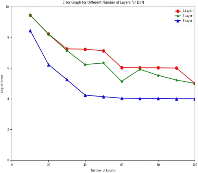

  

  Error graph for different number of layers for DBN

  Fig. 5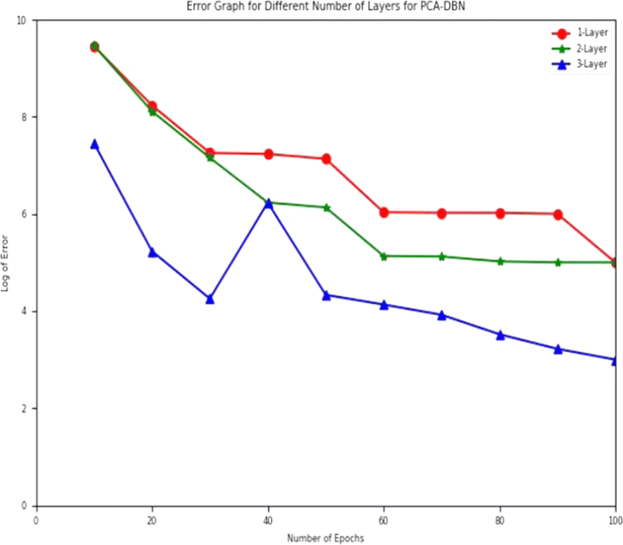

  

  Error graph for different number of layers for PCA-DBN

  Fig. 6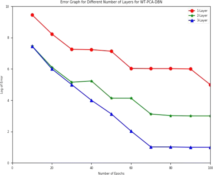

  

  Error graph for different number of layers for proposed DWT-PCA-DBN

• c. Weight initialization: Weights initialization is one of the most effective approaches in speeding up the training of a neural network. In fact, it influences not only the speed of convergence, but also the probability of convergence and the generalization. Using too small or too large values could speed the learning, but at the same time, it may end up performing worse. In addition, the number of iterations of the training algorithm and the convergence time would vary depending on the initialized values. In this phase of performance validation, considering weight initialization for all three individual deep learning based networks and other methods have been measured and given in Figs. 7, 8, 8 and 9. Three different initialization methods have been applied during the training of 100 epochs such as (a) small weights between 0 and 1 (b) large weights between 1 and 10 and (c) initializing with zero weights. For DBN network from Fig. 7, it can be seen that, initializing the weights of DBN network with all the types of random values results in converging from 40 epochs but experimenting with small random weights results in least error. PCA-DBN network as shown in Fig. 8 also shows better convergence and less error with respect to initializing the network with small weights. Similarly, in proposed DWT-PCA-DBN network shown in Fig. 9, experimenting with small values for weight initialization helps the network with least error, though, it converges at 70 epochs. While comparing among all three networks from Fig. 10, it can be concluded that, proposed DWT-PCA-DBN network for image classification is showing outstanding performance with respect to the number of epochs and error. DBN network is converging at 40 epochs, while PCA-DBN is at 100 epochs and DWT-PCA-DBN is 70 epochs with least error in comparison to other two networks.

  Fig. 7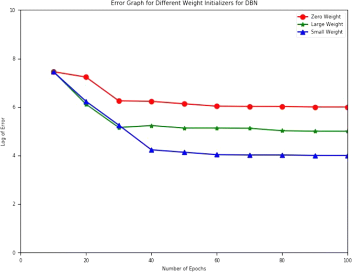

  

  Error graph for different weight initialization methods for DBN

  Fig. 8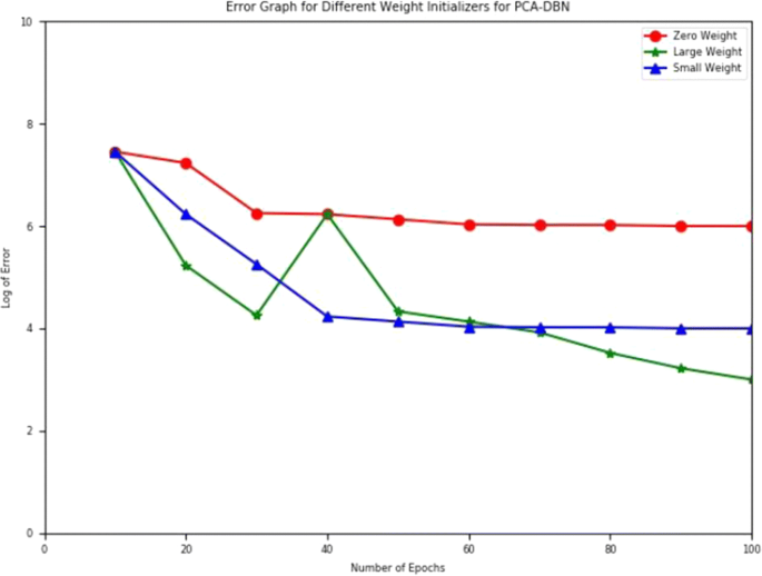

  

  Error graph for different number of layers for PCA-DBN

  Fig. 9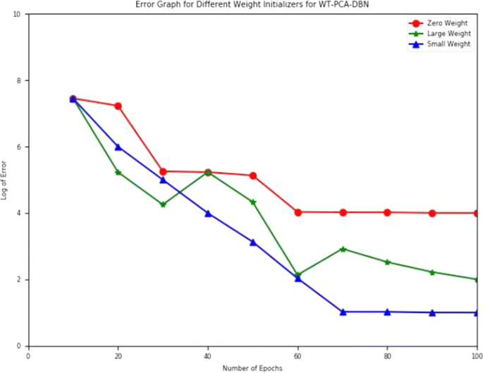

  

  Error graph for different number of layers for proposed DWT-PCA-DBN

  Fig. 10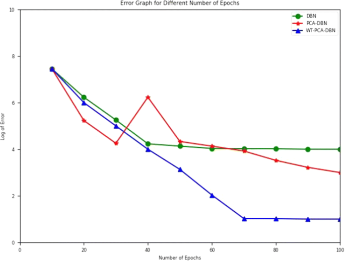

  

  Error graph for different techniques such as; DBN, PCA-DBN and proposed DWT-PCA-DBN

• d. Statistical analysis

  Two level statistical analysis such as McMemar’s test along with overall accuracy, average accuracy, and Kappa statistics for training sets and testing sets have been conducted for DBN, DWT-PCA and DWT-PCA-DBN as detailed below.

  • a. The McNemar’s test, which is based upon the standardized normal test statistic, is used to demonstrate whether the two methods perform differently in the statistical sense. The statistic is computed using (7).

    $$MN_{ij} = \frac{{mn_{ij} - mn_{ji} }}{{\sqrt {mn_{ij} + mn_{ji} } }}$$

    (7)

    where, $mn_{ij}$ denotes number of samples misclassified by I classifier but not by j classifier. Similarly $mn_{ji}$ denotes number of samples misclassified by j classifier but not by I classifier. This is basically derived from the Chi squared distribution using (8).

    $$\chi^{2} = \frac{{\left( {b - c} \right)^{2} }}{{\left( {b + c} \right)}}$$

    (8)

    Under the null hypothesis $mn_{ij}$ is equal to $mn_{ji}$. That is equivalent to the number of counts for (9).

    $$mn_{ij} = mn_{ji} = {\raise0.7ex\hbox{${(mn_{ij} + mn_{ji} )}$} \!\mathord{\left/ {\vphantom {{(mn_{ij} + mn_{ji} )} 2}}\right.\kern-0pt} \!\lower0.7ex\hbox{$2$}}$$

    (9)

    At 95% level of confidence, the difference of accuracies between the two methods (DBN and DWT-PCA-DBN) is significant as | $mn_{ij}$ | = 3.841 which is greater than 1.96. Hence the null hypothesis can be rejected. Similarly at 95% level of confidence the difference of accuracies between the two methods (DWT-DBN and DWT-PCA-DBN) is significant as | $mn_{ji}$ | = 2.147 which is greater than 1.96. Hence, the null hypothesis can be rejected and the alternative hypothesis can be accepted that states there is a significant difference between the corresponding two different classifiers.

• b. Measuring the overall accuracies (OAs), average accuracies (AAs), and Kappa statistics (Kappa) of ten run of trainings and tests of DWT, PCA-DBN and DWT-PCA-DBN (Table 4).

  Table 4 Performance comparison based on overall accuracies, average accuracies, and Kappa statistics for DBN, DWT-DBN and proposed DWT-PCA-DBN

The following are few observations of the current study that makes it challenging and interesting for image classification.

• a. In this study, RIDER Neuro MRI data which contains imaging data on 19 patients with recurrent glioblastoma who underwent repeat imaging sets have been extensively used and experimented.

• b. To deal with the large dataset, a local cloud server with high end configurations and also with GPU support and Python has been used for experimentation.

• c. To compare the performances among several settings, the DBN has been trained with various parameters and structures and computed the results of training and testing errors for each scenario.

• d. To compare the performance with other classification techniques, various performance measurement metrics such as classification accuracy, specificity, sensitivity and F-score are being measured.

• e. A comparative result has been obtained between deep learning and non-deep learning based strategies and from Table 2, it can be observed that, proposed deep learning based proposed DWT-PCA-DBN image classification model is showing significantly improved result over non deep learning based methods.

• f. The performance comparison has also been established among traditional DBN, DWT-DBN and DWT-PCA-DBN and it can be concluded from Table 3 that, the performance of DWT-PCA-DBN is more as compared to other techniques as deep learning approach is more efficient for image classification task and also the DWT-PCA-DBN technique outperforms the general DBN as there are more streamlining of feature selection has been done through DWT-PCA approach.

• g. Considering the number of epochs required for training the RBN network, from Fig. 4 it can be observed that, layer 3 gradually decreases from 40 till 100 numbers of epochs showing much better performance, similarly, from Figs. 5 and 6, it is seen that, layer 3 converges at 50 epochs and 70 epochs for PCA-DBN and DWT-PCA-DBN image classifiers, respectively.

• h. Therefore, while comparing the convergence of all three networks with respect to number of epochs and errors occurred, it can be concluded that proposed DWT-PCA-DBM is showing best setting with optimal value of error and epochs.

• i. As the weight initialization is one of the important factor considered during network initialization and tuning, in this work, three weight initialization ranges have been considered for all three deep learning based networks.

• j. For DBN network as shown in Fig. 7, it can be seen that, initializing the weights of DBN network with all the types of random values results in converging from 40 epochs but experimenting with small random weights results in least error.

• k. PCA-DBN network as shown in Fig. 8 also shows better convergence and less error with respect to initializing the network with small weights.

• l. Similarly, in proposed DWT-PCA-DBN network shown in Fig. 9, experimenting with small values for weight initialization helps the network with least error, though, it converges at 70 epochs.

• m. While comparing among all three networks from Fig. 10, it can be concluded that, proposed DWT-PCA-DBN network for image classification is showing outstanding performance with respect to the number epochs and error. DBN network is converging at 40 epochs, while PCA-DBN is at 100 epochs and DWT-PCA-DBN is 70 epochs with least error in comparison to other two networks.

• n. Additionally, statistical performance measures have been performed using McNemar’s test to validate the significant differences between the different existing and proposed classifier models.

Conclusion and future scope

Deep learning is well known approach for image classification as it is able to automatically extract the features from image data for further processing. However, the correctness of the extracted features is not guaranteed because there is no mathematical validation available for the correctness of those extracted features. To address this issue, this study proposed an improved DWT-PCA-DBN image classifier based image classification model by combining DWT for feature extraction and PCA to get optimized features with DBN. The DBN is composed of stacked RBMs to extract the more significant features from the reduced datasets layer by layer. Generally, DBN requires huge and multiple hidden layers with huge number of hidden units to learn the best features from the raw pixels of image data. This actually increases the complexity as well as training time for the model. Therefore, by integrating DBN with wavelet transform techniques both complexity as well as training time has been reduced. Except using raw images, the extracted low resolution images from DWT are used for training the proposed image classifier. The proposed model has been experimented with deep learning based approaches such as traditional DBN, PCA-DBN with non-deep learning based approaches of variants of ANN and also the performance of the proposed classifier has been evaluated based on number of epochs for training of RBN and weight initialization. Finally, the statistical validation justifies the efficiency of this method. The work can be extended to improve the computation efficiency of the model with respect to large amount of dataset with occlusion kind of patterns. Occlusion generally refers the blockage of blood flow into the brain. This type of pattern may occur in a tumor spot. This is also a kind of abnormality which may need attention for proper diagnosis. In this work we have not experimented our model for tumors with occlusion kind of pattern due to the unavailability of such patterns in the data. However, the work can be extended upon the availability of data with occlusion patterns using deep learning methods.

References

Glioblastoma Tumor: https://www.abta.org/tumor_types/glioblastoma-gbm/. Accessed 08 Nov 2019.
Jaiswal AK, Tiwari P, Kumar S, Gupta D, Khanna A, Rodrigues JPC. Identifying pneumonia in chest X-rays: a deep learning approach. Measurement. 2019;145:511–8.
Khatami A, Khosravi A, Nguyen T, Lim CP, Nahavandi S. Medical image analysis using wavelet transform and deep belief networks. Expert Syst Appl. 2017;86:190–8.
Gao X, Li W, Loomes M, Wang L. A fused deep learning architecture for viewpoint classification of echocardiography. Inf Fus. 2017;36:103–13.
Gao XW, Hui R, Tian Z. Classification of CT brain images based on deep learning networks. Comput Methods Programs Biomed. 2017;138:49–56.
Affonso C, Rossi ALD, Vieira FHA, Carvalho AC. Deep learning for biological image classification. Expert Syst Appl. 2017;85:114–22.
Qayyum A, Anwar SM, Awais M, Majid M. Medical image retrieval using deep convolutional neural network. Neurocomputing. 2017;266:8–20.
Litjens G, Kooi T, Bejnordi BE, Setio A, Ciompi F, Ghafoorian M, Laak J, Ginneken B, Sánchez C. A survey on deep learning in medical image analysis. Med Image Anal. 2017;42:60–88.
Gao X, Li W, Loomes M, Wang L. A fused deep learning architecture for viewpoint classification of echocardiography. Information Fusion. 2017;36:103–13.
Sharma H, Zerbe N, Klempert I, Hellwich O, Hufnagl P. Deep convolutional neural networks for automatic classification of gastric carcinoma using whole slide images in digital histopathology. Comput Med Imaging Graph. 2017;61:2–13.
Rahhal M, Bazi Y, AlHichri H, Alajlan N, Melgani F, Yager RR. Deep learning approach for active classification of electrocardiogram signals. Inf Sci. 2016;345:340–54.
Tang Q, Liu Y, Liu H. Medical image classification via multiscale representation learning. Artif Intell Med. 2017;79:71–8.
Zhong P, Gong Z, Li S, Schonlieb C. Learning to diversify deep belief networks for hyperspectral image classification. IEEE Trans Geosci Remote Sens. 2017;55:3516–30.
Zhao Z, Jiao L, Zhao J, Gu J, Zhao J. Discriminant deep belief network for high-resolution SAR image classification. Pattern Recogn. 2017;61:686–701.
Wang G, Qiao J, Li X, Wang L, Qian X. Improved classification with semi-supervised deep belief network. IFAC-PapersOnLine. 2017;50(1):4174–9.
Shi C, Pun C. Super pixel-based 3D deep neural networks for hyperspectral image classification. Pattern Recogn. 2018;74:600–16.
Paoletti ME, Haut JM, Plaza J, Plaza A. A new deep convolutional neural network for fast hyperspectral image classification. ISPRS J Photogramm Remote Sens. 2018;145(A):120–47.
Barboriak D. Data from RIDER_NEURO_MRI. The Cancer Imaging Archive. 2015. http://doi.org/10.7937/K9/TCIA.2015.VOSN3HN1.
Acknowledgements
Prayag Tiwari has received funding from the European Union’s Horizon 2020 research and innovation program under the Marie Sklodowska-Curie Grant Agreement No 721321.
This work is financially supported by the Ministry of Science and Higher Education of the Russian Federation (Government Order FENU-2020-0022).
Funding
The research received no external funding.
Author information
Authors and Affiliations
Contributions
AVNR, CPK, PKM, SKS and PT prepared the draft and Idea. AVNR, CPK performed the programming. PKM, SKS and PT analyzed the results. SK and MZ wrote the manuscript prepared the tables, references and checked the English. All authors read and approved the final manuscript.
Corresponding author
Ethics declarations
Competing interests
The author declare no competing interests in publication of this article.
Additional information
Publisher's Note
Springer Nature remains neutral with regard to jurisdictional claims in published maps and institutional affiliations.
Rights and permissions
Open Access This article is licensed under a Creative Commons Attribution 4.0 International License, which permits use, sharing, adaptation, distribution and reproduction in any medium or format, as long as you give appropriate credit to the original author(s) and the source, provide a link to the Creative Commons licence, and indicate if changes were made. The images or other third party material in this article are included in the article's Creative Commons licence, unless indicated otherwise in a credit line to the material. If material is not included in the article's Creative Commons licence and your intended use is not permitted by statutory regulation or exceeds the permitted use, you will need to obtain permission directly from the copyright holder. To view a copy of this licence, visit http://creativecommons.org/licenses/by/4.0/.
About this article
Cite this article
Reddy, A.V.N., Krishna, C.P., Mallick, P.K. et al. Analyzing MRI scans to detect glioblastoma tumor using hybrid deep belief networks. J Big Data 7, 35 (2020). https://doi.org/10.1186/s40537-020-00311-y
Received:
Accepted:
Published:
DOI: https://doi.org/10.1186/s40537-020-00311-y