Leveraging machine learning and big data for optimizing medication prescriptions in complex diseases: a case study in diabetes management

Abstract

This paper proposes a novel algorithm for optimizing decision variables with respect to an outcome variable of interest in complex problems, such as those arising from big data. The proposed algorithm builds on the notion of Markov blankets in Bayesian networks to alleviate the computational challenges associated with optimization tasks in complex datasets. Through a case study, we apply the algorithm to optimize medication prescriptions for diabetic patients, who have different characteristics, suffer from multiple comorbidities, and take multiple medications concurrently. In particular, we demonstrate how the optimal combination of diabetic medications can be found by examining the comparative effectiveness of the medications among similar patients. The case study is based on 5 years of data for 19,223 diabetic patients. Our results indicate that certain patient characteristics (e.g., clinical and demographic features) influence optimal treatment decisions. Among patients examined, monotherapy with metformin was the most common optimal medication decision. The results are consistent with the relevant clinical guidelines and reports in the medical literature. The proposed algorithm obviates the need for knowledge of the whole Bayesian network model, which can be very complex in big data problems. The procedure can be applied to any complex Bayesian network with numerous features, multiple decision variables, and a target variable.

Introduction

Motivation

Complex datasets arise in many disciplines, including health care, business, and engineering. In problems involving data-driven optimization based on such complex datasets, it is difficult to characterize optimality. The difficulty results from the many variables in the data (including nonmodifiable features as well as modifiable decision variables) and the numerous sources that generate the data at high speed. The complexity of a dataset might affect the optimization task since relevant features might fail to be matched, and considerations of all combinations of the decision variables might yield a computationally intractable problem. By leveraging machine learning (ML) and big data, we propose a new algorithm that identifies the optimal decision variables that affect the target variable while matching the relevant features. The proposed algorithm builds on the markov blanket (MB) and the associated d-separation property in Bayesian network (BN) models. We apply the algorithm to the management of patients who have comorbidities (i.e., multiple coexisting diseases) and take several comedications (a.k.a. polypharmacy). It is quite challenging to identify the optimal combination of medications for these patients.

Approaches such as outcome-based prescribing and individualized comparative effectiveness attempt to provide patients with the best set of medication recommendations based on what has worked for similar patients [1,2,3]. Many researchers have highlighted the need for comparative effectiveness studies to improve patient outcomes [4,5,6,7,8]. Data for conducting outcome-based prescribing are available, but the method of analysis is not clear, and various suggested methods have led to contradictory findings [9, 10]. Through a case study, we use type 2 diabetes (T2D) to test the proposed algorithm and its applications in complex disease management. We demonstrate how the optimal combination of diabetic medications can be found by examining the comparative effectiveness of a small, yet statistically sufficient, subset of medications among similar patients. In this article, we use polypharmacy and comedication interchangeably.

Outcome-based prescribing for management of patients with comorbidities and comedications

The main idea in outcome-based prescribing is to characterize similar cases. One would expect that, at a minimum, a similar case in the dataset will match (i.e., share) diagnoses with the patient at hand. However, limiting the matching to patients with the same diagnoses is not an easy task. For example, a polypharmacy patient may have $q$ diagnoses and take $q$ medications, and each medication could have $m$ alternatives. This suggests that outcomes must be examined for ${2}^{q \times m}$ combinations of medications and diagnoses. When $q$ and $m$ are large numbers, which is the case in big data, the analysis becomes cumbersome. Our proposed solution is to rule out those features and decision variables that are irrelevant in optimizing the target variable of interest.

An example of such complex problems is the management of patients with T2D. Diabetes is a public health problem affecting 400 million patients worldwide. The risks of death and cardiovascular events among diabetic patients are two to four times greater than those risks in the general population [11]. Moreover, controlling diabetes is crucial in delaying cardiovascular complications [12].

In this study, we propose a novel algorithm to address the above complexity problem by showing how a BN, learned from data, can be used for large scale data-driven optimization. BNs can model the stochastic and complex relationships among features, decision variables, and target variables. Moreover, in these models, the concepts of MB and the associated d-separation property can be used for each decision variable to identify the variables outside the blanket that are statistically independent of the target variable, given the knowledge of variables inside the blanket [13, 14]. We use this property to overcome dimensionality challenges with data-driven optimization in complex datasets.

Related works

In this section, we review the relevant research published mostly after 2015. This literature includes (1) management of polypharmacy for patients with comorbidities, (2) applications of ML/Artificial Intelligence (AI) in disease management for patients with polypharmacy and/or comorbidity, (3) overall applications of ML/AI in diabetes management, and (4) exclusive applications of BNs in disease management.

Management of polypharmacy for patients with comorbidities is an active area of research in the medical community. The studies within this research stream focus mainly on predicting clinical outcomes or investigating the effectiveness of combinations of medications. Wami and associates [15] used logistic regression to predict HbA1C (the average level of blood sugar as a measure of diabetes status) among T2D patients with comorbidity and comedications. Their study confirmed the potential impact of coexisting diseases and multiple medications on the efficacy of treatment and highlighted the research gap in developing treatment policies that take both factors into account. Research groups led by Utz and Ruzicka [16, 17] investigated the difficulty of treatment for patients with Gaucher disease Type 1 and chronic hepatitis C virus, respectively. Both studies emphasized the need to optimize medication treatment strategies for such complex diseases. Indu et al. [18] conducted a descriptive study that investigated the role of polypharmacy and comorbidity in the treatment of T2D. They also underlined the excessive complexity of treating T2D patients and called for more research on identifying the appropriate drug combinations for these patients.

The complexity of disease management in the presence of comorbidity and polypharmacy has been the focus of studies based on data analytics using ML/AI. For example, Keine and colleagues [19] investigated the effect of polypharmacy on older adults with dementia or Alzheimer’s disease and predicted the medication burden using ML. Other investigators [20,21,22] raised computational challenges with predicting the effects of drug combination (both synergism and antagonism) and suggested ML as an effective method for tackling the challenge when data are available. A recent review article [23] that assessed the applications of ML/AI in drug combinations revealed that most studies focus on predictive analytics (e.g., predicting the outcomes of drug combinations) as opposed to prescriptive analytics (e.g., optimizing the combinations of drugs). It also reported limited applications of BNs compared with other ML/AI methods.

There is also an extensive literature on the applications of ML/AI in diabetes management. A recent seminal paper by Dankwa-Mullan et al. [24] reviewed more than 450 articles (published between 2009 and 2018) to investigate the role of ML/AI in transforming diabetic care. Despite overall success with the use of ML/AI in diabetic care, the article reported inadequate attention to the treatment aspects of diabetes management or BN applications. In another recent review article, Contreras and Vehi [25] considered 141 articles published between 2010 and 2018. Their study highlights the complexity of diabetes management and the need to optimize therapeutic decisions, and concludes with confidence in a growing and promising use of ML/AI methods for diabetes management. It also notes that the prediction and prevention of the diabetes-related complications are the dominant topics, while treatment optimization has been explored less. Their review article supports our observation that BNs have not been used widely for diabetes management.

Finally, we instigated the applications of BNs in disease management. BNs have been successfully used in the treatment of cancer [26, 27] and cardiovascular disease [28]. Among the few papers assessing the applications of BNs for diabetes management, is the one by Sambo and associates, who used BNs for probabilistic reasoning and imputing missing risk factors in T2D [29]. Chamaria et al. [30] investigated the control of blood cholesterol level using monotherapy among patients with T2D. Finally, Porta et al. [31] employed BNs to investigate the relationships between epigenetic, cytokine, and endocrine variables in patients with T2D. None of these articles use BNs for treatment optimization.

The most noticeable gap in the body of the literature discussed above is treatment optimization for patients with complex diseases involving comorbidities and comedications. We fill this gap by proposing a data-driven algorithm for disease management, which (a) can handle the complexity arising from big health care data in the presence of coexisting diseases and multiple medications, and (b) can be used efficiently to optimize complex treatment decisions. To our knowledge, this is the first study that utilizes the MB property of BNs to optimize treatment decisions in a complex health care problem.

Materials and method

In this section, first, we provide an overview of the technical background required for this study. Next, we present our proposed method, followed by a description of the dataset that we used in our experimental study.

Technical background

A Bayesian network (BN) captures all dependence and independence relationships among a set of random variables in a compact network graph. Variables are the nodes of the network, and the arcs between the nodes imply the dependence/independence relationships among those variables. All nodes leading directly to an individual node are its “parents” and the nodes that directly follow it are its “children.” Following the arrowheads in a BN, a node is dependent only on its parents. More specifically, a node is independent of all other ancestors (i.e., the parents of its parents) conditional on the adjacent parent nodes. Such conditional independence leads to simple and compact factorization of the joint probability distribution of the entire network. In order for a BN to be represented by such compact joint probability factorization, the network must be acyclic (depicted by a Directed Acyclic Graph, referred to as DAG), meaning that the arrows leaving a node cannot return to it [32]. More formally, a BN model denoted by $BN = \left( {{\mathcal{X}},{\mathcal{E}}} \right)$ is a set of all nodes (captured in the set ${\mathcal{X}}$) and all edges (captured in the set $\varepsilon$) of the model. In such a network, the joint probability distribution of the entire network can be factorized as follows:

$$\begin{array}{*{20}c} {\Pr \left( {\mathcal{X}} \right) = \mathop \prod \limits_{n = 1}^{N} \Pr \left( {X_{n} |pa\left( {X_{n} } \right)} \right)} \\ \end{array}$$

(1)

where ${\mathcal{X}} = \left\{ {X_{1} , \ldots ,X_{N} } \right\}$ is the set of all $N$ variables indexed by $n$, and $pa\left( {X_{n} } \right)$ denotes the set of parents of the random variable $X_{n}$.

The independence relations in a BN can be captured in the Markov Blanket (MB) of a node, denoted by $MB\left( {X_{n} } \right)$. The MB of a node identifies the smallest subset of the variables around it (i.e., inside the blanket), conditional on which the node becomes independent of all other variables in the network (i.e., outside the blanket). Graphically, $MB\left( {X_{n} } \right)$ consists of parents, children, and co-parents (i.e., parents of the children) of $X_{n}$. The $MB\left( {X_{n} } \right)$ d-separates $X_{n}$ from all other nodes in ${\mathcal{X}}$; otherwise, they are said to be d-connected [13, 33]. Figure 1 illustrates the MB of a node inside a BN.

Fig. 1

Bayesian network (a) versus Markov blanket (b)

While the graph on the left shows a complete BN of a problem with ${\mathcal{X}} = \left\{ {D_{1} , X_{1} , \ldots ,X_{7} } \right\}$, the subgraph on the right illustrates the Markov blanket of the variable $D_{1}$. One can observe that the network of $MB\left( {D_{1} } \right)$ is more parsimonious than the whole BN as it includes two fewer random variables and seven fewer edges. The resulting parsimony translates into not only fewer computations needed for calculating the conditional and joint probabilities of the network but also more computationally tractable optimizations around $D_{1}$. This is because (a) the number of computations needed to characterize the joint/conditional probabilities grows exponentially with the number of node and edges, and (b) the computations for characterizing the optimal value of the decision variables (such as $D_{1}$) become less tractable with the growth in the number of features to be matched and the number of decision variables to be examined around $D_{1}$. The resulting computational efficiency becomes more prominent when dealing with complex datasets such as the ones arising from big data. We capitalize on this simplification for optimizing decision-making in complex problems.

In the above example, the joint probability distribution of the entire network can be factorized as follows:

$$\begin{array}{*{20}c} {\Pr \left( {\mathcal{X}} \right) = \Pr \left( {X_{1} ,X_{2} , \ldots ,X_{7} , D_{1} } \right)} \\ \end{array}$$

(2)

$$= \Pr \left( {X_{1} } \right)\Pr \left( {X_{2} |X_{1} } \right)\Pr \left( {X_{3} |X_{1} } \right)\Pr \left( {X_{4} |X_{2} ,D_{1} } \right)\Pr \left( {X_{5} |X_{3} ,X_{4} ,X_{6} ,D_{1} } \right)\Pr \left( {X_{6} |X_{2} ,X_{4} } \right)\Pr \left( {X_{7} |X_{5} ,X_{6} } \right)\Pr \left( {D_{1} |X_{1} } \right)$$

However, a variable of interest, e.g., $D_{1}$, can be fully characterized by a simplified proportionality relationship in the $MB\left( {D_{1} } \right)$ as follows:

$$\begin{array}{*{20}c} {\Pr \left( {D_{1} |X_{1} ,X_{2} , \ldots ,X_{7} } \right) \propto \Pr \left( {X_{4} |X_{2} ,D_{1} } \right)\Pr \left( {X_{5} |X_{3} ,X_{4} ,D_{1} } \right)\Pr \left( {D_{1} |X_{1} } \right)} \\ \end{array}$$

(3)

where the equality holds with a normalization constant independent of $D_{1}$ [34].

The elegance of the MB concept, which plays a key role in our proposed algorithm, is that it includes sufficient information for calculating the probability distribution of the node [13]. In other words, to fully characterize a node within a network, we only need information about the MB of that node, because, by definition, all other information (i.e., outside the MB) becomes irrelevant.

In the context of our case study, we define the set of all variables as ${\mathcal{X}} = \left\{ {{\mathcal{F}},{\mathcal{D}},\text{ }M} \right\}$, where ${\mathcal{F}}$ denotes the set of feature variables (i.e., the diagnoses and patient characteristics), ${\mathcal{D}}$ denotes the set of decision variables (i.e., medications), and $M$ denotes the target variable (i.e., mortality). Therefore, we utilize the d-separation property based on the features in ${\mathcal{F}}$ that d-separate the decision variable in ${\mathcal{D}}$ from the target variable $M$. In the next subsection, we show how we use this property to identify the smallest subset of variables that affect the relationship between the decision variables and the target variable, thereby reducing the complexity of the optimization task.

Proposed method

The main idea behind our proposed algorithm is that if a BN can be characterized, then d-separation can be used to identify a handful of relevant features that affect the impact of the decision variables on the target variable. However, not all elements within the MB of the decision variable can be controlled by the decision-maker. For example, the clinician cannot modify the patient’s demographics. Therefore, similar cases within the dataset should be restricted to cases that match these features of the case at hand. Diagnoses can be treated in two ways, depending on whether they are the cause for taking medication (i.e., $Diagnosis \to Medication$) or side effects of the medication (i.e., $Medication \to Diagnosis$). A diagnosis cannot change by itself. Therefore, all similar cases should share the diagnoses in the MB that lead to the selection of the patient’s medication. We denote by ${\mathcal{F}}_{1k}$ the set of features pointing to medication $D_{k}$. The MB may also contain diagnoses that result from the use of medication. Although clinicians can prescribe different medications and modify doses, they cannot control medication effects. Therefore, the consequence of these medications cannot be fixed as this is the mechanism through which the medications affect the risk of mortality. These diagnoses are allowed to vary and do not need to be matched. The set of features resulting from medication $D_{k}$ is denoted by ${\mathcal{F}}_{2k}$. Finally, there are typically several medications within $MB\left( {D_{k} } \right)$. These are the decision variables, the set of which is denoted by ${\mathcal{D}}_{k}$. The analysis needs to find their optimal combination leading to the minimum risk of mortality. In summary, the MB of decision variable $D_{k}$ consists of three sets of variables: the set of features that need to be matched (i.e., ${\mathcal{F}}_{1k}$), the set of features that do not need to be matched (i.e., ${\mathcal{F}}_{2k}$), and the set of decision variables ${\mathcal{D}}_{k}$. Their combinations have to be optimized with respect to the target variable $M$. In other words,

$$\begin{aligned} {if: MB\left( {D_{k} } \right) = \left\{ {{\mathcal{F}}_{1k} ,{\mathcal{F}}_{2k} ,{\mathcal{D}}_{k} } \right\}} \\ \text{then, optimal actions for particular realization of the feature set, denoted by}\; {\mathcal{F}}_{1}^{0}\; \text{will be}:\\ = \mathop {\text{argmin}}\limits_{c} \Pr \left( {M = 1|{\mathcal{F}}_{1k} = {\mathcal{F}}_{1}^{0} ,{\mathcal{D}}_{k} = {\mathcal{D}}_{k}^{c} } \right),\\\end{aligned}$$

(4)

where $M = 1$ indicates death and ${\mathcal{D}}_{k}^{c}$ indicates an instantiation of decision variables inside ${\mathcal{D}}_{k}$.

When different MBs share decision variables, contradictory optimal recommendations may arise. To resolve these conflicting recommendations, we merge the conflicting MBs and repeat the algorithm with the new MB. The mathematical interpretation of merging two MBs is simply to find their union set. This leads to the identification of the optimal recommendations based on the majority voting rule commonly used in ML [35, 36]. Figure 2 summarizes the proposed algorithm for optimizing a set of decision variables with respect to a target variable while matching the set of relevant features in a BN.

Fig. 2

The proposed algorithm for optimization of medication mix

The conflicting recommendations emerge when different optimal recommendations are suggested through different MBs. In other words, $V_{ij}^{*} \ne V_{{i^{\prime}j}}^{*}$ identifies conflicting optimal recommendations through $MB\left( {D_{i} } \right)$ and $MB\left( {D_{{i^{\prime}}} } \right)$ for the patient type $j$. To resolve this issue, we combine the conflicting MBs to create a virtual $MB\left( {D_{{i^{\prime\prime}}} } \right) = MB\left( {D_{i} } \right) \cup MB\left( {D_{{i^{\prime}}} } \right)$ and rerun the algorithm for $MB\left( {D_{{i^{\prime\prime}}} } \right)$ starting from step “A” in the proposed algorithm.

Source of data for experimental study

Dataset description and general preprocessing

This study examined data from the electronic health records of diabetic patients seen at the Washington DC Veterans Administration Medical Center. Each subject had different first and last visit dates. The average earliest visit date was April 2002, and the average latest visit date was June 2008. The first date of visit across all subjects was March 1998, and the last date of visit was May 2011. The analysis was conducted on 19,223 diabetic patients.

Eligibility criteria

The eligibility criteria for inclusion in the final dataset included the following:

• a. Diabetic: The patient must have had two diagnoses of diabetes in the past 2 years. A diagnosis of diabetes refers to any of the following International Classification of Disease codes: 250.xx, 357.2, 362.0x, 366.41 or 648.0x. The x in the following codes refers to any digit.

• b. Minimum data required: The first and last visits should be at least 180 days apart. Patients with fewer than 180 days between first and last visits were excluded on suspicion that they could have been receiving care elsewhere.

• c. Inconsistent date of death: Patients with a recorded date of death 30 days prior to their last visit were not included in the analysis. A 30-day interval was allowed because, occasionally, test results become available after the date of death or visits are coded to have been completed after the death date.

Among the diabetic patients examined, 17,773 (92.2%) met the eligibility criteria. We found no records with missing data.

Dependent variable

The primary target variable in this study was all-cause mortality. We focused on mortality because it provides an endpoint for all illnesses, not just those related to diabetes [37].

Independent variables

The independent variables included the following:

• 1. Severity of illness: Severity of illness was calculated from all patients’ diagnoses during the study period based on the procedure patented by Alemi and Walters [38] for the following set of complications: renal; diabetic; other endocrine; cardiac; hypoglycemic; digestive; circulatory; ear, nose, and throat; endocrine; eye; female reproductive; health care status; hematopoietic; hepatobiliary; HIV; infection; injury; kidney; male reproductive; mental; musculoskeletal; neoplasia; nerve; respiratory; skin; substance abuse; and other diseases.

• 2. Diabetic medications: This set of independent variables identified the diabetes medication that the patient was prescribed in the last year of care. These included the following: insulin, acarbose, chlorpropamide, dipeptidyl peptidase-4 (DPP4), glimepiride, glipizide, glyburide, metformin, pioglitazone, repaglinide, rosiglitazone, tolazamide, and troglitazone. For each medication, the prescribed daily dose (PDD) was calculated in the last year of care as the measure of the rate of use according to [39].

• 3. Demographics: Year of birth, gender, race, and ethnicity were used to characterize patient demographics.

Methods and dataset preprocessing for BN learning

To capture meaningful relationships between the variables in the BN, first, we introduced three classes of variables:

• 1. Root nodes (variables that could not be affected by other variables): Birth year, Hispanic, white, married, and male were preset as root nodes. They are highlighted in pink in the model (Fig. 3).

  Fig. 3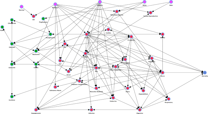

  

  Impact of diabetic medications on mortality

• 2. End node (variables that could not affect other variables): Mortality was set as the target variable and is represented by the blue spiral node in the model.

• 3. Intermediate nodes (variables that could be both the cause and effect of other variables): Medications and their various complications were set as intermediary nodes. They are presented as green nodes (diabetic medications) and red nodes (complications) in the model.

Next, the following sets of arcs were prohibited when building the BN: all arcs from the intermediate class to the root class, all arcs from the end class to the root class, and all arcs from the end class to the intermediate class.

Finally, we used a combination of Augmented Naïve Bayes [40, 41] and Taboo order [42] BN learning from data. We implemented the algorithm in the software application BayesiaLab version 5.0.6, using its supervised and unsupervised modules for BN learning and the Decision Tree Optimization module for the optimization task [43].

Results and discussion

BN model

The learning procedure resulted in a BN with a total precision of 88.75% and area under receiver operating characteristic curve (AUC) of 71.15% (using tenfold cross-validation), which together suggest an acceptable model fit. Figure 3 depicts the resulting BN constructed from data. It shows the impact of diabetic medications (green nodes on the left), demographic variables (pink nodes on the top), and severity of illness in various body systems (red nodes) on mortality (blue spiral node at the right). The network model shows a set of interesting relationships. For example, Hispanic ethnicity affects what medications are taken and whether patients are sicker, and severity of illness affects mortality directly, as it should. Also, the use of medications affects mortality through side-effects and severity of illness, which, again, makes intuitive sense.

Descriptive results

To examine the practical relevance of the BN model and to further motivate our proposed algorithm for treatment optimization, in this section, we present the results of simple descriptive analytics using the BN model. In doing so, we conducted the following conditional probability queries as a hard evidence analysis common in BN analysis [44]:

$$\begin{array}{*{20}c} {\Pr \left( {M = 1 |X_{n} = x_{n}^{c} } \right)} \\ \end{array}$$

(8)

where $M = 1$ represents death, $X_{n}$ is the variable of interest in the query and $x_{n}^{c}$ is the realization of interest for $X_{n}$.

The impact of demographics on mortality

Figure 4 illustrates the effect of demographic variables on the risk of mortality (i.e., $X_{n}$ in Eq. (8) is a demographic variable). On average, 12.28% of our diabetic patients died (the horizontal red line in all panels of Fig. 4). Being Hispanic increased mortality by 4.18% (from 11.03% for not being Hispanic, [the red bar] to 15.21% for being Hispanic [the green bar]). The increased risk of mortality among the US-born Hispanics has also been reported in other studies [45]. Younger patients survived longer than older ones, with mortality dropping to 4.35% for young patients versus 19.58% for older patients. The effect of aging on mortality is well established in the literature [46]. Marriage had a negligible effect on survival (as there is no significant difference between the two bars), which contradicts findings of other studies that suggested a protective effect for marriage [45, 47]. Being male increased mortality by 0.81%. The increased risk associated with being male has been reported in several studies [48,49,50], although some other studies have shown no difference [51,52,53]. Other demographic variables in our dataset did not affect the mortality rate.

Fig. 4

Impact of demographic variables on mortality

The impact of diabetic medications on mortality

Using our BN model, we conducted descriptive analytics to assess the impact of prescribing a medication on the risk of mortality (i.e., $X_{n}$ in Eq. (8) is a medication variable). Figure 5 shows the probability of mortality associated with diabetes medications in our data. The dashed line shows the apriori rate of mortality in the population examined, i.e., the rate that is expected for an average patient. Values below this line indicate that the medication might be protective and thus reduce the mortality rate to less than the average rate. The values above the line indicate the reverse. The range of values suggests that the extent to which the medications impact the mortality rate depends on other factors in the model. Most of our findings are aligned with the literature. For example, our results show that the use of insulin increases the probability of mortality by 1.4%, from 11.87% for little or no use to 13.27% for higher dosages (these figures correspond to the minimum and maximum height of the bar associated with insulin in the figure, respectively). The association between insulin use and mortality has been reported in the literature [54]. The use of rosiglitazone increased mortality by 5.43%. The association between the use of rosiglitazone and an increased risk of cardiovascular illness and sudden death has been reported in the literature [55]. The use of acarbose increased mortality by 1.99%. However, the use of glipizide reduced mortality by 0.36%. Higher rates of use of pioglitazone had a negligible effect on mortality. Recent studies have shown that pioglitazone might protect patients against some cardiovascular risks [56]. The use of glyburide increased mortality rate from 11.15% for patients with little or no use to 12.41% for patients with further use. This increase in mortality rate has also been reported in the literature [57]. The use of glimepiride decreased mortality from 12.98% for patients with little or no use to 12.28% for patients with further use. The literature suggests that the use of glimepiride might be associated with increased mortality risks [58]. The use of DPP4 decreased mortality to 12.13% compared with 12.28% for patients who did not use this medication. These findings have also been reported in the literature [59].

Fig. 5

Range of mortality for different medications

Despite the concordance between our findings and the literature, the reported impact of single medications largely depends on the patients’ conditions and the medications they are taking. The key takeaway is that for several medications, notably metformin, rosiglitazone, acarbose, insulin, and glyburide, the range of effect is dispersed both above and below the average mortality rate. This suggests that under certain conditions, these medications can both increase and decrease the risk of mortality. For example, since a major portion of the graph for metformin is below the horizontal line, this medication seems to be the most promising intervention for an average patient to reduce the risk of mortality. An important question, therefore, is how to distinguish patients who are likely to benefit from the medications from those who are not. More specifically, how do we find the best combination of medications for different patients? The question can be answered by running an exhaustive number of conditional probability queries and characterizing the optimal medication decisions for the patient group of interest. However, running all conditional probability queries of all mixes of medications for all combinations of feature variables can be computationally intensive and sometimes even intractable. This is particularly true for complex problems arising from big data. In the next section, we present the results of our proposed optimization algorithm for characterizing the optimal combination of diabetic medications among various patient types. As discussed earlier, the algorithm does not rely on the exhaustive list of conditional probability computations. Instead, the optimization task will be conducted on the set of statistically relevant features and medications identified through the MBs in the BN model.

Optimization results

In this section, we illustrate the results of our proposed optimization algorithm. Before presenting the results for all medications, we provide details regarding the implementation of the proposed algorithm, using metformin as an example.

An illustrative example

Suppose a young, Hispanic patient who is in good health status is using metformin. Would this patient’s outcomes be improved if he or she discontinues metformin or adds other medications? First, the BN allows us to predict the patient’s average risk of mortality, which is 2.14%. Notice that birth year, Hispanic ethnicity, glyburide, glipizide, rosiglitazone, insulin, health status, renal condition, and circulatory conditions are in the MB of metformin (in boldface type in Fig. 6). In other words, following the notations introduced previously, we have:

Fig. 6

Markov blanket of metformin

$$MB\left( {Metformin} \right) = \left\{ {{\mathcal{D}}_{Metformin} ,{\mathcal{F}}_{1,Metformin} ,\,{\mathcal{F}}_{2,Metformin} } \right\}$$

where:

$${\mathcal{D}}_{Metformin} = \left\{ {Glyburide,\,Glipizide, \,Rosiglitazone, \,Insulin} \right\}$$

$${\mathcal{F}}_{1,Metformin} = \left\{ {BirthYear, \,Hispanic, \,Status} \right\}$$

$${\mathcal{F}}_{2,Metformin} = \left\{ {Renal, \,Circulatory} \right\}$$

Therefore, all variables outside $MB\left( {Metformin} \right)$ are irrelevant to the decision, as they are d-separated from $Mortality$ by the variables inside the MB. On the $MB\left( {Metformin} \right)$, the variables belonging to ${\mathcal{F}}_{1,Metformin}$ (namely, Hispanic ethnicity, age, and health status) affect the selection of $Metformin$ (at they lead to it) and hence should be matched to the patient. The medications on the $MB\left( {Metformin} \right)$ (i.e., metformin, glyburide, glipizide, insulin, and rosiglitazone) are the decision variables and should be optimized with respect to mortality. Therefore, it is important that we examine the outcome for all possible combinations of these medications. This is accomplished using the decision tree optimization algorithm, which is based on finding the best medication combination among all possible combinations, taking the matched variables into account [43]. Our results show that the probability of mortality among patients who are Hispanic, young, and less sick is 2.28% (see the first column in Table 1). After implementing the optimization algorithm with $MB\left( {Metformin} \right)$, our results show that the optimal combination of medications for this patient type is metformin, no insulin, and no glipizide. This decision yields 2.13% as the minimum risk of mortality. In other words:

Table 1 Results of the proposed algorithm with all MBs in the data for selected patient types

$${\text{for }}i {\text{ and }}j {\text{ such that:}}\left\{ {\begin{array}{*{20}c} {\text{patient type: } P_{j} = \left\{ {BirthYear = young, \,Hispanic = yes, \,Status = low} \right\}} \\ {\text{Markov blanket:} \,D_{i} = Metformin} \\ \end{array} } \right.$$

The algorithm gives the following optimal solutions:

$${\text{Optimal action:}} \,V_{ij}^{*} = \left\{ {Metformin = 1, \,Insulin = 0, Glipizide = 0} \right\}$$

$${\text{Optimal outcome:}} \,m_{ij}^{*} = 2.13\%.$$

For the above patient type, the best treatment strategy is to use monotherapy with metformin, and this optimal action minimizes the patient’s risk of mortality to 2.13%.

Optimal medication recommendations

Table 1 summarizes the results of our proposed algorithm for all MBs of the medications in the data for a selected patient type based on the features in the set ${\mathcal{F}}_{1,medication}$. The table should be read column-wise. Each column identifies the results of analyses for each MB (column title) for the matched features in the MB (corresponding to the green rows) and the optimal medication decisions (corresponding to the yellow rows). The first orange row indicates the average risk of mortality before implementing the algorithm for the selected patient type specified through the corresponding matched variables. The second orange row indicates the minimum risk of mortality if the patient follows the optimal medication decisions identified in the column.

An interesting observation from the results of our algorithm is that only six features belong to the set ${\mathcal{F}}_{1}$ of all MBs. In other words, many features had no impact on the selection of the optimal medication combination. Clearly, this simplifies the optimization procedure significantly.

We extensively discussed the results for $MB\left( {Metformin} \right)$. The same optimal recommendation (i.e., monotherapy with metformin) is made for the selected patient (in column 7), who has high hypoglycemic and skin severities in addition to the characteristics of the patient in column 1. Indeed, monotherapy with metformin is the optimal medication for the selected patient types in columns 1, 2, 7, 8, and 10. Rosiglitazone alone is the optimal medication for a white patient with good health status (column 4). For the selected patients in columns 5 and 6 (i.e., an average patient), the optimal medication prescription is monotherapy with glipizide, whereas, for the selected patient in column 9, the optimal treatment is monotherapy with glyburide. Double therapy (metformin and pioglitazone) is recommended only for the patient in column 3. Other optimal recommendations could have been obtained if we had matched the selected patient with different states of the variables in the green rows. Column 10 shows the results of resolving conflicting recommendations between Columns 2 and 4. To resolve this conflict, we repeated the optimization procedure with the union of the two MB’s. The revised recommendation is now to use metformin only and stop using rosiglitazone.

One interesting observation is that metformin appeared more than all other medications, at least as a part of the optimal treatment recommendation. This is consistent with the descriptive results in Fig. 5, where metformin had the largest range of values below the horizontal line (i.e., positive effects in reducing mortality).

Our analysis relied on diabetes medications and not non-diabetic medications. When we include these decision variables, a much more complex BN model emerges (see the “Appendix”). The resulting network is a lot larger, and the MB for the medications is much more complex. Nevertheless, the procedure for analysis remains similar.

Concluding remarks

This paper demonstrates how a BN could help in optimal decision-making when facing complex problems such as those arising from big data. We propose an algorithm that takes advantage of the MB of the decision variables to identify matched features and the optimal combination of the decision variables. To our knowledge, this is the first study that utilizes the MB property of BNs for optimizing treatment decisions in a complex health care problem.

There is a concern that as data become more complex, computational difficulties will arise regarding characterizing optimal decisions while matching relevant features. Based on our proposed algorithm, however, even for very large datasets, with millions of records and thousands of variables, it is still possible to focus on cases that d-separate decision variables from the target variable. The key idea behind our proposed algorithm is that, in such circumstances, it is not necessary to know the full BN. Instead, we only need to know (a) the MB of each decision variable and (b) how controlling for the elements of the MB can alter the target variable. This is of great importance in the analysis of big data when a massive number of features and decision variables are generated through various sources at high speed.

Comparison with other methods

To better understand the value and novelty of our proposed method and its applications, we compared our study with two published studies.

First, we compared our proposed method with a previous analysis conducted on the same dataset by Kheirbek et al. [39]. That study used logistic regression to predict the effectiveness of diabetic medications in relation to all-cause mortality. Although the analysis can be used to estimate the conditional probabilities $\Pr \left( {M = 1 |X_{n} = x_{n}^{c} } \right)$, their predictive model does not capture the complex interactions among the variables in the data. In logistic regression, interaction can be included through various degrees of interaction terms, but this approach normally leads to computational challenges with model estimation and poor fit. Second, contrary to our proposed method, logistic regression does not provide a way to focus the computations on the smallest subset of variables linking decision variables to the target variable. Third, the study reported various results on the effectiveness of the medications, which are different from our results. For example, the earlier work found no effectiveness of metformin in reducing mortality, whereas our study suggests metformin as an optimal monotherapy for several patient groups. Our results are more consistent with the recommendation by the American Diabetes Association [60] and the conclusions of Mekuria and colleagues [61], which confirms the effectiveness of metformin monotherapy. One reason for such discrepancies between our study and [39] might be the failure of the logistic regression model to capture complex relationships among variables, leading to incomplete customization of the analyses to various patient types. Another reason might be the lack of optimization in their study. Interestingly, the authors highlighted such limitation as the most important step in advancing the research:

“Given the large number of hypoglycemic medications and comorbid conditions, it may be important to develop tools that can help selection of optimal medications for diabetic patients that present with comorbidities.”

Our proposed method fills the gap by providing optimal recommendations customized to the patient types.

The idea of foregoing construction of full BNs and focusing on the MB was also promulgated by Bai and colleagues [62]. While the direction of their work and ours is similar, there are major differences, particularly from an application perspective. The key difference is that Bai and colleagues did not employ MB for optimization purposes. Both approaches rely on MB, yet for different purposes and in different ways. They used MB around the target variable as a feature selection method to aid in predicting the target outcomes. Instead, we used MB of the decision variables to aid in optimizing their effect on the target variable. We relied on the MB property to understand what is relevant in controlling the impact of the decision variables on a target variable. The way we formulated the problem is similar to theories of relevance described by Hjørland and Christensen [62], where the relevance of a third variable is defined in the context of the relationship between two variables. This epistemological perspective argues that a variable is relevant (i.e., part of the MB, in our case) if it has an impact on the relationship between decision variables and the target variable.

Theoretical and clinical implications

Our study has both theoretical and managerial implications. On the theoretical side, it has suggested an efficient algorithm that facilitates data-driven optimization with complex datasets. The value of such simplification becomes more eminent in large scale optimizations with big data, where the complexity of the computations grows exponentially with the number of variables in the feature and decision sets. On the health care management side, the proposed algorithm can be used to optimize data-driven treatment decisions in complex diseases. Other examples of complex diseases include hypertension [64] and cancer [65], where multiple treatment alternatives (mainly combination therapy) exist for various patient types under different patient adherence scenarios.

Limitations and future work

A great deal of characterizing the comparative effectiveness of medications from big data remains uninvestigated. We have not shown the optimal solution when we use all medications (diabetic and non-diabetic) reported in the data. Future research should focus on optimal ways of deriving individualized comparative effectiveness in the presence of both sets of medications. We were also limited by a relatively small sample size (n = 19,223). Given that ML methods perform better with large datasets and optimization tasks become more complicated with big data, a larger set of data would likely better illustrate the utility of our proposed method.

Appendix A: BN for non-diabetic medications

The following image shows the complexity of the analysis when the non-diabetic medications are included in the analysis. See Fig. 7.

Fig. 7

Bayesian network with both diabetic and non-diabetic medications

References

Lee JD, Nunes EV Jr, Novo P, Bachrach K, Bailey GL, Bhatt S, et al. Comparative effectiveness of extended-release naltrexone versus buprenorphine-naloxone for opioid relapse prevention (X: BOT): a multicentre, open-label, randomised controlled trial. Lancet. 2018;391:309–18.
Wang Z, Whiteside SP, Sim L, Farah W, Morrow AS, Alsawas M, et al. Comparative effectiveness and safety of cognitive behavioral therapy and pharmacotherapy for childhood anxiety disorders: a systematic review and meta-analysis. JAMA Pediatr. 2017;171:1049–56.
Mills KT, Obst KM, Shen W, Molina S, Zhang H-J, He H, et al. Comparative effectiveness of implementation strategies for blood pressure control in hypertensive patients: a systematic review and meta-analysis. Ann Intern Med. 2018;168:110–20.
O’Brien MJ, Perez A, Scanlan AB, Alos VA, Whitaker RC, Foster GD, et al. PREVENT-DM comparative effectiveness trial of lifestyle intervention and metformin. Am J Prev Med. 2017;52:788–97.
Lee SWH, Chan CKY, Chua SS, Chaiyakunapruk N. Comparative effectiveness of telemedicine strategies on type 2 diabetes management: a systematic review and network meta-analysis. Sci Rep. 2017;7:12680.
Suissa S. Lower risk of death with SGLT2 inhibitors in observational studies: real or bias? Diab Care. 2018;41:6–10.
Schneeweiss S, Seeger JD, Jackson JW, Smith SR. Methods for comparative effectiveness research/patient-centered outcomes research: from efficacy to effectiveness. J Clin Epidemiol. 2013;66:S1–4.
Derosa G, Sibilla S. Optimizing combination treatment in the management of type 2 diabetes. Vasc Health Risk Manag. 2007;3:665–71.
Green J, Czanner G, Reeves G, Watson J, Wise L, Beral V. Oral bisphosphonates and risk of cancer of oesophagus, stomach, and colorectum: case-control analysis within a UK primary care cohort. BMJ. 2010;341:c4444.
Cardwell CR, Abnet CC, Cantwell MM, Murray LJ. Exposure to oral bisphosphonates and risk of esophageal cancer. JAMA. 2010;304:657–63.
Rawshani A, Rawshani A, Franzén S, Eliasson B, Svensson A-M, Miftaraj M, et al. Mortality and cardiovascular disease in type 1 and type 2 diabetes. N Engl J Med. 2017;376:1407–18.
Reaven PD, Emanuele NV, Wiitala WL, Bahn GD, Reda DJ, McCarren M, et al. Intensive glucose control in patients with type 2 diabetes—15-year follow-up. N Engl J Med. 2019;380:2215–24.
Pearl J. Causal inference in statistics: an overview. Stat Surv. 2009;3:96–146.
Murphy KP. Machine learning: a probabilistic perspective (adaptive computation and machine learning series). USA: MIT Press; 2012.
Wami WM, Buntinx F, Bartholomeeusen S, Goderis G, Mathieu C, Aerts M. Influence of chronic comorbidity and medication on the efficacy of treatment in patients with diabetes in general practice. Br J Gen Pr. 2013;63:267–73.
Utz J, Whitley CB, van Giersbergen PL, Kolb SA. Comorbidities and pharmacotherapies in patients with Gaucher disease type 1: the potential for drug–drug interactions. Mol Genet Metab. 2016;117:172–8.
Ruzicka DJ, Tetsuka J, Fujimoto G, Kanto T. Comorbidities and co-medications in populations with and without chronic hepatitis C virus infection in Japan between 2015 and 2016. BMC Infect Dis. 2018;18:237.
Indu R, Adhikari A, Maisnam I, Basak P, Sur TK, Das AK. Polypharmacy and comorbidity status in the treatment of type 2 diabetic patients attending a tertiary care hospital: an observational and questionnaire-based study. Perspect Clin Res. 2018;9:139–44.
Keine D, Zelek M, Walker JQ, Sabbagh MN. Polypharmacy in an elderly population: enhancing medication management through the use of clinical decision support software platforms. Neurol Ther. 2019;8:79–94.
Sharma A, Rani R. An integrated framework for identification of effective and synergistic anti-cancer drug combinations. J Bioinform Comput Biol. 2018;16:1850017.
Vakil V, Trappe W. Drug combinations: mathematical modeling and networking methods. Pharmaceutics. 2019;11:E208.
Xia F, Shukla M, Brettin T, Garcia-Cardona C, Cohn J, Allen JE, et al. Predicting tumor cell line response to drug pairs with deep learning. BMC Bioinform. 2018;19:71–9.
Tsigelny IF. Artificial intelligence in drug combination therapy. Brief Bioinform. 2019;20:1434–48.
Dankwa-Mullan I, Rivo M, Sepulveda M, Park Y, Snowdon J, Rhee K. Transforming diabetes care through artificial intelligence: the future is here. Popul Health Manag. 2019;22:229–42.
Contreras I, Vehi J. Artificial intelligence for diabetes management and decision support: literature review. J Med Internet Res. 2018;20:e10775.
Bradley A, Van Der Meer R, McKay C. Personalized pancreatic cancer management: a systematic review of how machine learning is supporting decision-making. Pancreas. 2019;48:598–604.
Jiang X, Wells A, Brufsky A, Neapolitan R. A clinical decision support system learned from data to personalize treatment recommendations towards preventing breast cancer metastasis. PloS ONE. 2019. https://doi.org/10.1371/journal.pone.0213292.
Loghmanpour NA, Kanwar MK, Druzdzel MJ, Benza RL, Murali S, Antaki JF. A new Bayesian network-based risk stratification model for prediction of short-term and long-term LVAD mortality. ASAIO J. 2015;61:313–23.
Sambo F, Facchinetti A, Hakaste L, Kravic J, Di Camillo B, Fico G, et al. A Bayesian network for probabilistic reasoning and imputation of missing risk factors in type 2 diabetes. In: Holmes JH, Bellazzi R, Sacchi L, Peek N, editors. Artif Intell Med. Cham: Springer International Publishing; 2015. p. 172–6.
Chamaria S, Johnson KW, Vengrenyuk Y, Baber U, Shameer K, Divaraniya AA, et al. Intracoronary imaging, cholesterol efflux, and transcriptomics after intensive statin treatment in diabetes. Sci Rep. 2017;7:1–13.
Porta M, Amione C, Barutta F, Fornengo P, Merlo S, Gruden G, et al. The co-activator-associated arginine methyltransferase 1 (CARM1) gene is overexpressed in type 2 diabetes. Endocrine. 2019;63:284–92.
Kjærulff UB, Madsen AL. Bayesian Networks and Influence Diagrams: A Guide to Construction and Analysis. 2nd ed. Springer; 2012.
Pearl J. Causality: Models, Reasoning and Inference. 2nd ed. Cambridge University Press; 2009.
Korb KB, Nicholson AE. Bayesian artificial intelligence [Internet]. CRC press; 2010 [cited 2016 Jul 12]. Available from: https://books.google.ca/books?hl=en&lr=&id=LxXOBQAAQBAJ&oi=fnd&pg=PP1&dq=Nicholson+AE.+Bayesian+artificial+intelligence&ots=Q1WG9bh2D5&sig=-khUK5bYwxirxpBBzRof-QmDUY0.
Milosevic N, Dehghantanha A, Choo KKR. Machine learning aided android malware classification. Comput Electr Eng. 2017;61:266–74.
Randhawa K, Loo CK, Seera M, Lim CP, Nandi AK. Credit card fraud detection using AdaBoost and majority voting. IEEE Access. 2018;6:14277–84.
Sohn M-W, Arnold N, Maynard C, Hynes DM. Accuracy and completeness of mortality data in the Department of Veterans Affairs. Popul Health Metr. 2006;4:2.
Alemi F, Walters SR. A mathematical theory for identifying and measuring severity of episodes of care. Qual Manag Health Care. 2006;15:72–82.
Kheirbek RE, Alemi F, Zargoush M. Comparative effectiveness of hypoglycemic medications among veterans. J Manag Care Pharm. 2013;19:740–4.
Husmeier D, Dybowski R, Roberts S. Probabilistic modeling in bioinformatics and medical informatics. Springer Science & Business Media; 2006.
Ripley BD. Pattern recognition and neural networks. New york: Cambridge University Press; 2008.
Friedman N, Nachman I, Pe’er D. Learning Bayesian network structure from massive datasets: the “sparse candidate” algorithm. arXiv:13016696. 2013.
Conrady S, Jouffe L. Bayesian networks and bayesiaLab: a practical introduction for researchers. USA: Bayesia; 2015.
Fenton N, Neil M. Risk Assessment and decision analysis with Bayesian networks. Boca Raton: Chapman and Hall/CRC; 2018.
Dey AN, Lucas JW. Physical and mental health characteristics of US-and foreign-born adults: United States, 1998–2003. Adv Data. 2006;369:1–19.
Caspersen CJ, Thomas GD, Boseman LA, Beckles GL, Albright AL. Aging, diabetes, and the public health system in the United States. Am J Public Health. 2012;102:1482–97.
Manzoli L, Villari P, Pirone GM, Boccia A. Marital status and mortality in the elderly: a systematic review and meta-analysis. Soc Sci Med. 2007;64:77–94.
Ghali JK, Piña IL, Gottlieb SS, Deedwania PC, Wikstrand JC. Metoprolol CR/XL in female patients with heart failure analysis of the experience in metoprolol extended-release randomized intervention trial in heart failure (MERIT-HF). Circulation. 2002;105:1585–91.
Gustafsson F, Torp-Pedersen C, Burchardt H, Buch P, Seibaek M, Kjøller E, et al. Female sex is associated with a better long-term survival in patients hospitalized with congestive heart failure. Eur Heart J. 2004;25:129–35.
Simon T, Mary-Krause M, Funck-Brentano C, Jaillon P. Sex differences in the prognosis of congestive heart failure: results from the Cardiac Insufficiency Bisoprolol Study (CIBIS II). Circulation. 2001;103:375–80.
Lee WY, Capra AM, Jensvold NG, Gurwitz JH, Go AS. Gender and risk of adverse outcomes in heart failure. Am J Cardiol. 2004;94:1147–52.
Opasich C, Tavazzi L, Lucci D, Gorini M, Albanese MC, Cacciatore G, et al. Comparison of one-year outcome in women versus men with chronic congestive heart failure. Am J Cardiol. 2000;86:353–7.
Sheppard R, Behlouli H, Richard H, Pilote L. Effect of gender on treatment, resource utilization, and outcomes in congestive heart failure in Quebec, Canada. Am J Cardiol. 2005;95:955–9.
Schramm TK, Gislason GH, Vaag A, Rasmussen JN, Folke F, Hansen ML, et al. Mortality and cardiovascular risk associated with different insulin secretagogues compared with metformin in type 2 diabetes, with or without a previous myocardial infarction: a nationwide study. Eur Heart J. 2011;32:1900–8.
Nissen SE, Wolski K. Rosiglitazone revisited: an updated meta-analysis of risk for myocardial infarction and cardiovascular mortality. Arch Intern Med. 2010;170:1191–201.
Shah P, Mudaliar S. Pioglitazone: side effect and safety profile. Expert Opin Drug Saf. 2010;9:347–54.
Pantalone KM, Kattan MW, Yu C, Wells BJ, Arrigain S, Jain A, et al. The risk of overall mortality in patients with type 2 diabetes receiving glipizide, glyburide, or glimepiride monotherapy a retrospective analysis. Diab Care. 2010;33:1224–9.
Pantalone KM, Kattan MW, Yu C, Wells BJ, Arrigain S, Nutter B, et al. The risk of overall mortality in patients with type 2 diabetes receiving different combinations of sulfonylureas and metformin: a retrospective analysis. Diab Med. 2012;29:1029–35.
Dicembrini I, Pala L, Rotella CM. From theory to clinical practice in the use of GLP-1 receptor agonists and DPP-4 inhibitors therapy. Exp Diab Res. 2011;2011(2011):898913.
American Diabetes Association. Standards of medical care in diabetes—2017 abridged for primary care providers. Clin Diab. 2017;35:5–26.
Mekuria AN, Ayele Y, Tola A, Mishore KM. Monotherapy with metformin versus sulfonylureas and risk of cancer in type 2 diabetic patients: a systematic review and meta-analysis. J Diab Res. 2019. https://doi.org/10.1155/2019/7676909.
Hjørland B, Christensen FS. Work tasks and socio-cognitive relevance: a specific example. J Am Soc Inf Sci Technol. 2002;53:960–5.
Bai X, Padman R, Ramsey J, Spirtes P. Tabu search-enhanced graphical models for classification in high dimensions. Inf J Comput. 2008;20:423–37.
Zargoush M, Gumus M, Verter V, Daskalopoulou SS. Designing risk-adjusted therapy for patients with hypertension. Prod Oper Manag. 2018;27:2291–312.
Ayer T, Alagoz O, Stout NK, Burnside ES. Heterogeneity in women’s adherence and its role in optimal breast cancer screening policies. Manag Sci. 2015;62:1339–62.
Acknowledgements
The authors thank the editorial team and the ten reviewers for their helpful comments. The manuscript was copyedited by Linda J. Kesselring, MS, ELS.
Funding
Not applicable.
Author information
Authors and Affiliations
Contributions
MZ led the research project. MM and MZ contributed to the algorithm design, analysis, interpretation of data, and drafting of the manuscript. FA contributed to the acquisition of data, analysis, algorithm design, interpretation of data, and drafting of the manuscript. RK contributed to the acquisition of data, analysis, interpretation of data, and drafting of the manuscript. All authors read and approved the final manuscript.
Corresponding author
Ethics declarations
Ethics approval and consent to participate
Consent for publication
The authors grant the sole license of the full copyright in the contribution and guarantee that the contribution to the work has not been previously published elsewhere.
Competing interests
The authors declare no competing interests.
Additional information
Publisher's Note
Springer Nature remains neutral with regard to jurisdictional claims in published maps and institutional affiliations.