- Research
- Open access
- Published:
Spatial data extension for Cassandra NoSQL database
Journal of Big Data volume 3, Article number: 11 (2016)
Abstract
The big data phenomenon is becoming a fact. Continuous increase of digitization and connecting devices to Internet are making current solutions and services smarter, richer and more personalized. The emergence of the NoSQL databases, like Cassandra, with their massive scalability and high availability encourages us to investigate the management of the stored data within such storage system. In our present work, we harness the geohashing technique to enable spatial queries as extension to Cassandra query language capabilities while preserving the native syntax. The developed framework showed the feasibility of this approach where basic spatial queries are underpinned and the query response time is reduced by up to 70 times for a fairly large area.
Background
The proliferation of mobile applications and the widespread of hardware sensing devices increase the streamed data towards the hosting data-centers. This increase causes a flooding of data. Taking benefits from these massive dataset stores is a key point in creating deep insights for analysts in order to enhance system productivity and to capture new business opportunities. The inter-connected systems are sweeping almost all sectors forming what’s called today Internet of Things. These changes will have a big impact in the foreseeable future. Estimations say that the economic share of the internet of things will reach 11 % of the world economy by 2025 [1]. From the human health and fitness supervising, passing by smart-grids supply chains control and reaching intelligent transportation systems (ITS) monitoring, the generated data is becoming more and more context-oriented. Indeed, embedded applications send data associated to a location and time information. In ITS, for instance, the moving vehicles and the road side units (RSU) will be continuously broadcasting traffic-related and location-tagged packets. The produced data are underpinning different kinds of applications such as safety related, traffic efficiency and value-added services. The huge size of received and stored datasets might be more or less homogeneous. Moreover, data could be either structured or semi-structured. The data handling requirements are beyond the capabilities of the traditional data management systems. The community are currently aware of the added-value that could be derived from processing and analyzing big datasets. Surveys showed that less than 1 % of data are currently used for real-time control and a good opportunity for performance and prediction might be addressed using the remaining data [1]. Different frameworks are being investigated to deal with these new requirements at the storage layer, but also at the processing, analysis and visualization layers.
As an illustration of the data scale, data collected in the ITS for example by a single RSU could exceed 100 GB per day [2]. Hence, for a city or a country-scale deployment we could easily reach the petabyte scales in the first year. The management of this data requires innovating models. The NoSQL Not only SQL data management systems are standing for these new challenges. Indeed, Cassandra [3], MongoDB [4], Neo4J [5] and Redis [6] are, among others, too much dealt with in the research and business communities in the last period. A quick look on Google trends [7] comparing NoSQL versus RDBMS shows clearly the trends of both terms.
These new promising NoSQL solutions are not really suited for transaction queries so far. Indeed, the integrity model of data in the relational database systems assured by atomicity, consistency, integrity, and durability (ACID) proprieties is not possible to be applied when scaling out data. Regarding the NoSQL databases, it was proven that a database could have maximum two out of the consistency, availability, partition-tolerance proprieties (CAP) [8].
In this work, we are investigating a missing feature in Cassandra NoSQL database which is the spatial data indexing and retrieval. Indeed, most of this category of databases are not supporting geospatial indexes and hence spatial queries [8].
Our research contribution in this paper could be summarized as follows; We index stored data using geohashing technique [9] by converting the latitude/longitude information to a numeric geohash attribute and associate it to the data when being stored. Then, we develop a spatial query parser and define a spatial syntax as a Cassandra query language (CQL) spatial extension. Besides, since our lookup is based on the geohash attributes, we develop an aggregation algorithm for optimizing the number of queries to be routed to the cluster nodes. Finally we illustrate the new capability enabled in Cassandra and evaluate the response time to client spatial queries using different schemes: sequential, asynchronous and with and without queries aggregation.
This paper is organized as follows. the next section presents the related work. The section after is focusing on describing the system architecture and detailing the proposed approach. A benchmarking setup and performance evaluation are presented and discussed in the fourth section. We wrap up this paper with a conclusion and perspectives in the last section.
Related work
It is currently admitted that conventional relational databases are no longer the efficient option in a large and heterogeneous data environment. Alternatively, NoSQL technologies are showing better capabilities when uprising to petabyte scale and the system is partitioned. Indeed, the continuous growth of the data repositories hits the borders of the existing relational data management systems. Many other factors are driving users to fully or partly migrate and join the NoSQL emerging solutions including lack of flexibility and rigid schema, inability to scale out data, high latency and low performance, high support and maintenance costs [8].
The spectrum of the NoSQL is getting larger and several solutions are currently in place and being enhanced day after day. So far, they can fit into one of four sub categories of databases: document-stored, wide-column stored, key-value stored and graph oriented. Several differences and similarities exist regarding the design and features, the integrity, the data indexing, the distribution and the underlying compatible platforms [8]. Conducting analytics over big multidimensional data is another challenge that should be investigated within the context of NoSQL and big data emerging technologies [10].
Spatial search integration and data modeling in conventional databases used to be a hot topic since a while [11]. Currently, several conventional RDBMS and some NoSQL databases integrate geospatial indexing [8, 12]. Used techniques for geospatial indexing differ from one product to another. For instance, Galileo is a distributed hash table implementation where the geoavailability grid and query bitmap techniques are leveraged to distribute data within groups of nodes and to evaluate queries in order to reduce search space. The group membership and bitmap indexes are derived from the binary string of the geohashes. These techniques show better performance compared to the R-tree especially for big data retrieval [13]. However, The impact of partitioning algorithm in Galileo is different of the partitioning in Cassandra. Indeed, the random partitioning algorithm in Cassandra has a direct impact on the data retrieval queries. Hence, the grouping of nodes based on a specific criteria to store geographically closer events is not doable. Another scalable scheme proposed in [14] named VegaGiStore using multi-tier approach to store, index and retrieve spatial data within big data environment. The approach is based on MapReduce paradigm to distribute and parallelize the query processing. The performance of the scheme shows good results against conventional RDBMS such as PostGIS and Oracle Spatial. However, it remains a theoretical concept since no product has been publicly released [15].
System architecture and proposed approach
The classical relational databases show their limitations facing the inevitable data set size, information connectivity and semi structured incoming data leading to sparse tables [8]. Cassandra DB could be an appropriate candidate to handle the data storage with the aforementioned characteristics. The challenge in this choice is the missing of spatial query feature within Cassandra query language (CQL). An overview of Cassandra and CQL along with the proposed approach to extend its capabilities are discussed in the following subsections.
Cassandra DB and CQL
Cassandra is fully distributed, share nothing and highly scalable database, developed within Facebook and open-sourced on 2008 on Google code and accepted as Apache Incubator project on 2009 [16]. Cassandra DB is built based on Amazon’s Dynamo and Google BigTable [3]. Since that, continuous changes and development efforts have been carried out to enhance and extend its features. DataStax, Inc. and other companies provide customer support services and commercial grade tools integrated in an enterprise edition of Cassandra DB. Cassandra clusters can run on different commodity servers and even across multiple data centers. This propriety gives it a linear horizontal scalability. Figure 1 depicts an example of a possible physical deployment of Cassandra cluster, however, a logical view of the cluster is much more simple. Indeed, the nodes of the cluster are seen as parts of a ring where each node contains some chunks of data. The rows of data are partitioned based on their primary key. This latter could be composed from two parts: the first is called \(partition\ key\) based on it the hash function of the partitioner picks the receiving node to store data. The second part of the key is reserved for clustering and sorting the data within a given partition. A good spreading of data over a cluster should make a balance between two apparently conflicting goals [17]:

Overview of a physical cross data centers Cassandra cluster. A Cassandra cluster deployment over three datacenters and in multiple racks. The client could connect to the cluster through any node of the cluster called coordinator node
-
Spread data evenly across the cluster nodes;
-
Minimize the number of partitions read.
Spreading data evenly requires a fairly high cardinality in the partition key and the hash function output space. However, since data is scattered by partitions within the cluster nodes set, having a wide range of partition keys may lead to visiting more nodes for even simple queries and as a result, longer query response delay. In the opposite side, reducing too much the number of partitions may affect the load balancing between nodes and create hot-spot nodes degrading their responsiveness.
The philosophy behind Cassandra is different from a traditional relational database. Indeed, the need for a fast read and write combined with huge data handling are primordial in Cassandra. Hence, normalizing the data model by identifying the entity/relationship entities are not top priorities. However, designing the data access pattern and the queries to be executed against the data are more valuable in the data model design [17]. With this perspective, the data model accepts generally redundancy and denormalization of stored data and allows the storage of both simple primitives data types and composed data types such as collections (list, set, map). Recently, CQL gives the user the ability to extend the native data types with customized user data types (UDT). Even though these UDTs are stored as blobs strings in the database, they could be formatted, parsed and serialized within the client side using the custom codec interface [18].
The CQL version 3 offers a new feature of user defined functions (UDF). It’s a user defined code that can be run into Cassandra cluster. Once created, a UDF is added to cluster schema and gossiped to all cluster nodes. The UDFs are executed on queries result set in the coordinator node row by row. Aggregations over result set rows are also possible. Leveraging the UDFs to filter results returned by Cassandra engine at different nodes is still a challenging task. Indeed, the intention of the UDF feature developers was to delegate a light treatment at the cluster level on resulted rows. So far no possibilities to filter based on a user defined reference or value are available. Extending UDFs with this feature adds more flexibility of their usage and enables pushing some computation blocks from the client to the cluster side.
Geohashing and spatial search
The geohash is a geocoding system which consists in mapping latitude/longitude to a string by interleaving bits resulting from latitude and longitude iterative computation. The resulting bitstring is split into substrings of 5-bit length and mapped to 32-base character dictionary. Finally, a string of an arbitrary length is obtained which represents a rectangular area. The longer the geohash string, the higher is the precision of the rectangle. The successive characters represent nested addresses that converge to around 3.7 by 1.8 cm for 12 characters geohash string length [19]. For the best of our knowledge, Cassandra DB and its query language CQL don’t support spatial queries. Even though the literature presents some generic indexing and search libraries, such as Lucene-based elasticsearch [20] and Solr [21] java libraries. In this contribution, we tried to leverage the geohash technique to label and efficiently retrieve Cassandra stored rows within a user defined area of interest. This behavioral extension of Cassandra and CQL is illustrated in Fig. 2 which details the spatial data storage and retrieval phases accomplished through the following three steps:

Flowchart of the proposed approach for spatial data storage and retrieval. The flowchart depicts the sequence of actions and processes to store and retrieve spatially tagged data
-
First, every row, when being stored, is labeled with a numeric geohash value computed based on its latitude/longitude values. The computing of numeric geohash is required in the proposed approach because of the limitation of CQL in terms of operators applied on the String type. Indeed, the WHERE clause of native CQL presents only equality operators for textual types. However, the range queries are not possible. Events associated to a zone may be addressed in a future work.
-
Second, the queried area is decomposed into geohashes of different precision levels. Indeed, the biggest geohash box that fits into the queried area is the first to be computed. Then, the remaining area is filled with smaller geohashes until they are fully covering the area of interest. Since range query is not straight-forward within space-filling Z-order curve [22], a query aggregation algorithm for grouping neighbor geohashes is developed so that the number of generated queries is optimized.
-
Finally, the original query, defined via a new spatial CQL syntax is decomposed to a number of queries and executed sequentially or in parallel before aggregating result sets and returning them to the client.
Let’s further explain the above steps. We assume that in a Cassandra cluster database, the stored data scheme is under the form of events generated from distributed connected devices or external systems. The events are time-stamped and location-tagged. During the storage phase, the event’s timestamp and location are parsed to extract day, month, year and compute the corresponding numeric geohash (\(gh\_numeric\)). The event is stored and these attributes are passed as primary key attributes: day as partition key, month and year as clustering keys and \(gh\_numeric\) as either part of clustering keys or a secondary indexed column value. The definition of a such primary key is efficient in this specific-context where events are looked-up generally within time ranges and area of interest. In different context, the primary key structure may be different while being inline with Cassandra pattern data model design. The conversion of geohash value from its string representation to numeric representation enables querying ranges of events based on their \(gh\_numeric\) attributes. Indeed, since geohash values represent rectangles rather than exact geopoints location, the binary string of the geohash value is appended in the right side with a string of ‘0’ to get the \(min\_value\) and and a list of ‘1’ to get the \(max\_value\) representing the south–west and north-east rectangle corners values, respectively. Every location within this bounding rectangle has a \(gh\_numeric\) between \(min\_value\) and \(max\_value\). Hence, the spatial range query is reduced to a numeric range query instead of string-based query (which is allowed by CQL).
As depicted in Fig. 3, the binary representation of string geohash is extended with list of 0 or 1 to a predefined bit-depth to get respectively the geohash \(min\_value\) and \(max\_value\). For example, the ths geohash has a binary representation over 15 bits (each character is mapped to 5 bits). If we consider the binary extension is done over 52 bits, the geohash value has respectively a \(min\_value\) = 3592104487944192 and a \(max\_value\) = 3592241926897663. With this approach, each geohash that fits inside ths bounding box, will have a geohash numeric value between the \(min\_value\) and \(max\_value\). Nevertheless, the queries are not always over perfectly adjacent and ordered fences. A queried area could be of an arbitrary shape and the list of covering geohashes are of different precision.

Geohash and computing of numeric geohash values
Once a spatial query is received from the user, the original query is decomposed into sub-queries based on the resulting Gehashes bounding boxes. The number of resulting queries might be relatively high which may increase the query response time. To reduce the number of queries, a query aggregation algorithm is developed, Algorithm 1, and its integration in the query path is illustrated in Fig. 4.

The main function of the algorithm is the optimization of the generated sub-queries to be sent to the cluster and search space reduction. The optimization is derived from the removal of redundant bounding boxes or nested ones. For example, if a geohash is contained in another one, the upper one is kept and the smallest is removed because the result will be in the query of the containing geohash as depicted in Fig. 5a. Also, geohashes of same length could be reduced to a single geohash if their union fills its total content as illustrated in Fig. 5b. The last step is the aggregation of neighbor geohashes that could not be reduced to an upper geohash because they partly fill its content or may belong to different upper geohashes but they keep a total order of their global \(min\_value\) and \(max\_value\); This means that no other geohash, belonging to the list of geohashes to be aggregated and not grouped yet, belongs to the range limited by \(min\_value\) and \(max\_value\). This latter case is illustrated in the Fig. 5c where the green area composed of seven geohashes are aggregated into three ordered sets (yellow, orange, and purple). At this stage, queries could be sent to the coordinator nodes based on the partition key in either parallel or sequential scheme.

Queries aggregation algorithm for optimizing generated queries to be sent to Cassandra cluster

Geohashes aggregation scenarios. a Remove nested geohahses. b Groupe geohashes to an upper geohash. c Aggregate ordered geohashes into sets
Spatial search queries
For analytics purpose, several types of spatial queries could be looked up. Some of them cover simple area shapes, others may target more complicated ones. In the following, we pick up the basic three queries which can be seen as a base to compute others. But let’s first define the table on which we are going to write queries:

In this schema, \(gh\_numeric\) is part of the clustering key where Cassandra creates an index over it by default. Following, we consider three examples of spatial queries:
-
Around_me looking on a focal point is a recurrent scenario. Events around an important point of interest where no predefined geometric shape is known could be discovered by only giving a geocode location and a range or radius of circle centered at the point of interest. Fine or coarse grained lookup could be adjusted through the radius value and resulting output are retrieved accordingly. For discovery and update purposes, querying events around a location gives a 360° view of surrounding area. Following is a spatial query illustration of \(Around\_me\) type where SFUNC represents the spatial function taking two parameters; the first is a of String type defining the query type. The second parameter \(circle\_params\) is a container (list) of center coordinates, radius length and a maximum geohash precision value:

-
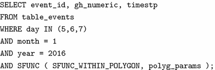
In a given area predefined zones like countries, districts or municipalities are subject of frequent queries in a spatial database context. Also non-predefined areas such as arbitrary polygon zones could be queried. Interested scientists may want to quantify, aggregate and visualize statistics of some criteria in the supervised area. By providing a list of geocode locations forming a closed polygon, our present framework cares of the rest. The following query example illustrates such syntax where \(polyg\_params\) is a container of list of latitude/longitude pairs and a maximum geohash precision length:
-
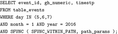
In my path another type of spatial queries may be of particular importance is within a road segment, in the path of a tracked vehicle or maybe in a traffic stream. Trying to limit the path with a polygon may be not the best option. Hence, providing way-points and a precision level of search could be more self-explained. This kind of queries may be very useful for analytics purposes but also for real time support of emergency fleets. An example of \(In\ my\ path\) query syntax is following where \(path\_params\) is a container of list of waypoints coordinates and geohash precision value:


The syntax is simple and intuitive and it conserves the native CQL syntax, which means native non-spatial queries could be executed either directly or through the developed spatial framework.
Performance evaluation
This section describes the environment of testing and discusses the results.
Benchmark settings and dataset
In this paper we carried out our work with community distribution of Datastax Cassandra v3.0.0 and with the Datastax java driver v3.0.0-beta1. The hosting machines are 5-nodes cluster of 4GB of RAM running Ubuntu 14.04.1 LTS server instances. Three different data sets with respectively 100 MB, 500 MB and 1 GB sizes are generated over the \(Umm\ Slal\) municipality in Qatar as depicted in Fig. 6. In fact, the whole municipality is decomposed to geo-fences of different precision lengths and generated events are attached to every geohash for different dates with a maximum precision value equal to 9 which means an accuracy of around 4.78 by 4.78 m [19] and minimum precision value equal to 6, around 1.2 by 0.61 km. It’s also worth to mention the usage of available open-source libraries exposing geographic utilities such as geotools [23] and guava [24] java libraries. We aim proving the feasibility of our approach to allow retrieving events within arbitrarily geometric defined fences, to measure their times of execution and to discover the impact of the stored data size on the spatial framework performance.

Umm Slal municipality map in Qatar
Results and discussion
In this section, we evaluate the different scenarios of query execution for previously selected three spatial queries: Circle, Path and in a given Polygon. We focus as well on the performance of the queries aggregation algorithm in terms of reduction of the number of queries sent to the cluster nodes.
Aggregation algorithm performance
Figure 7 shows the execution time required by the spatial query pre-processing phase to group and aggregate the geohashes covering the target area of the query. The graph illustrates the variation of both geohashes generation time and geohashes aggregation time for different precision levels (geohash length) against the queried area of the target zone (radius of circular zone). Values are reduced by log scale for the homogeneity of the graph. We could clearly notice that geohashes generation time variation is correlated with variation of the aggregation time. Indeed, for small areas, the execution time is reduced to few milliseconds regardless the required precision. However, the execution time goes upward when increasing the lookup area and the precision level. This increase could be explained by the way the algorithm is proceeding to compute the geohashes covering the queried area and the time complexity of the developed algorithm. The borders of the circular area need higher time to define the required precision and to identify the geohashes fully fitting into the area from others totally or partially fitting outside the border.

Geohashes aggregation algorithm performance. Execution time of both geohashes generation and aggregation for different precision (geohash length) levels and different circular areas measurement
In Table 1, the efficiency of the algorithm was assessed through quantification of reduction of queries routed to the coordinator node in the cluster from client application. A circular area is queried with different radius length values and a given precision. Results show that up to 73 % of queries could be reduced and thus avoid to make bottleneck in the cluster with a flooding of queries.
Spatial queries execution time
This subsection assesses the different scenarios of executing a spatial query within the present framework. Indeed, several spatial queries have been run and different combinations of CQL queries and geohashes aggregation algorithm are used. The queries are executed against different data set sizes. The averaged execution time over several hits of each query are recorded in Tables 2, 3 and 4 for respectively 100 MB, 500 MB and 1 GB data sets.
All the aforementioned tables depict the execution time of spatial queries over a circular area with different radius values going from few meters up to 10 km. All the scenarios are with a fixed precision value of 9. The output values show the out-performance of the asynchronous queries scheme versus the sequential one. Indeed, the asynchronous model decreases drastically the overall needed time to retrieve the result set. Besides, The execution of the aggregation algorithm over the set of geohashes to be queried outperforms the execution time and reduces as well the number of queries sent toward Cassandra cluster. The continuous increase of the target area increases the queries generation and aggregation time as already learned from the above aggregation performance graph. Hence, the spatial query execution time for asynchronous queries with aggregation may exceed the non-aggregated scenario when reaching big areas, 10 km circle radius length, for instance. Nevertheless, it’s still lower than the sequential scenario regardless using aggregation or not. As a learned lesson, it is recommended to use asynchronous model all the time. However, special care should be given to the advantages (reducing the sent queries to the cluster and avoid making hotspot nodes) and the cost (longer execution time) of using the aggregation algorithm especially when dealing with big areas.
Tables 5, 6 and 7 present the execution time of a queried path. The compared query schemes are also different combinations of sequential, asynchronous and with or without aggregation algorithm. The shape of the queried area is simple and the framework is able to quickly generate and aggregate the resulting geohashes. As a result, the impact of aggregation and asynchronous scenario is more clear in terms of response time reduction. This enhancement in response time is identified for all the tested paths. Indeed, for 10 km-long path, the query response time is around 38 times faster when using spatial aggregation and asynchronous queries. Another observation which is almost valid to all the tested spatial queries is the limited impact of the data set size. Indeed, one of the fundamental propriety of Cassandra is that it scales linearly by simply adding commodity server nodes. Hence, the developed framework scales well with the data set size.
Finally, the spatial polygon-based query in the developed framework is evaluated are results are given in Tables 8, 9 and 10. Measurement results are averaged over several executions for different polygon dimensions and with different geohash precision values. The spatial queries have been executed as well against different data set sizes. It’s then clear the enhancement of the response time by using the asynchronous mode and executing the spatial aggregation algorithm compared to other schemes. By focusing on the column \(AS\_AGG\), for asynchronous with aggregation, an effective time reduction of about 70 times is noticed against a normal scenario not using these enhancement features. The increase of the queried area keeps the asynchronous model with aggregation showing the best performance and this is due to the regular, rectangular, shape of the area.
Conclusion
This paper tackles the spatial data retrieval within Cassandra NoSQL database. For this goal, a framework is designed and implemented to extend the CQL with spatial queries. Indeed, a CQL-like syntax is defined to enable spatial functions while keeping the native CQL query syntax. The developed framework is tested against different data set sizes. The evaluation outcomes confirm the efficiency of using an aggregation algorithm in order to reduce the number of queries sent to the cluster and avoid making hot-spot nodes, despite its extra cost in terms of execution time. The importance of paralleling queries in non-blocking way to avoid unnecessary idle time is also highlighted through the performance results.
A learned lesson is that irregular area shapes might cause a longer time to compute the covering geohashes and to aggregate them. In this case, the user is invited to make decision based on its interest in either speeding up the query execution time or reducing the number of routed queries to the cluster.
We believe that presented framework could be a basic component of the big data system that we are building to support the data collection and management for the connected vehicles and distributed devices managed by Qatar Mobility Innovations Center (QMIC).
In our perspectives, we plan to extend Cassandra with two features: The first one is to enable the table creation query defining the attributes based on them numeric geohashes should be computed as part of the schema. The second one is to add the ability to generate numeric geohashes for already saved data in the background compaction process.
References
Manyika J, Chui M, Bisson P, Woetzel J, Dobbs R, Bughin J, Aharon D. McKinsey Global Institute —the internet of things: mapping the value beyond the hype. http://www.mckinsey.com/insights/business_technology/the_internet_of _things_the_value_of_digitizing_the_physical_world. Accessed 01 Mar 2016.
Drira W, Filali F. Ndn-q: an ndn query mechanism for efficient v2x data collection. IEEE 11th annual international conference on sensing, communication, and networking workshops (SECON Workshops); 2014
Lakhshman A, Malik P. Cassandra: a decentralized structured storage system. ACM SIGOPS Operating Syst Rev. 2010;44(2):35–40.
MongoDB, WG.: MongoDB. https://www.mongodb.org/. Accessed 1 Mar 2016
Robinson I, Webber J, Eifrem E. Graph databases: new opportunities for connected data. Sebastopol: O’Reilly Media; 2015.
Redis WG. Redis. http://redis.io/. Accessed 1 Mar 2016.
Google WG. Google trends. https://www.google.fr/trends/explore#q=NoSQL%2C%20RDBMS&cmpt=q&tz=Etc%2FGMT-3. Accessed 1 Mar 2016.
Moniruzzaman AB, Hossain SA. Nosql database: new era of databases for big data analytics—classification, characteristics and comparison. Int J Database Theor Appl. 2013;6(4):1–13.
Geohash WG. Geohash. https://www.en.wikipedia.org/wiki/Geohash. Accessed 1 Mar 2016.
Cuzzocrea A, Song IY, Davis KC. Analytics over large-scale multidimentional data: the big data reveolution. Glasgow: DOLAP’11; 2011.
Samet H, Aref WG. Spatial data models and query processing. Modern database systems: the object model, interoperability, and beyond. Reading: Addison Wesley/ACM Press; 1994.
Oracle WG. Oralce spatial developer’s guide. https://www.docs.oracle.com/cd/E11882_01/appdev.112/e11830/toc.htm. Accessed 1 Mar 2016.
Malensek M, Pallickara S, Pallickara S. Polygon-based query evaluation over geospatial data using distributed hash tables. UCC ’13 Proceedings of the 2013 IEEE/ACM 6th international conference on utility and cloud computing; 2013. p. 219–226.
Zhong Y, Han J, Zhang T, Li Z, Fang J, Chen G. Towards parallel spatial query processing for big spatial data. IEEE 26th International parallel and distributed processing symposium workshops and PhD forum; 2012.
Arnold T. An entropy maximizing geohash for distributed spatiotemporal database indexing. arXiv:1506.05158v1 [cs.DB]; 2015
Tutorialspoint WS. Cassandra—Introduction. http://www.tutorialspoint.com/cassandra/cassandra_introduction.htm. Accessed 1 Mar 2016.
Hobbs T. Basic rules of Cassandra data modeling. http://www.datastax.com/dev/blog/basic-rules-of-cassandra-data-modeling. Accessed 1 Mar 2016.
Datastax WG. Basic rules of Cassandra data modeling. https://www.datastax.github.io/java-driver/features/custom_codecs/. Accessed 1 Mar 2016.
ElasticSearch WG. Geohashes. https://www.elastic.co/guide/en/elasticsearch/guide/current/geohashes.html. Accessed 1 Mar 2016.
ElasticSearch WG. Elastic Java API. https://www.elastic.co/guide/en/elasticsearch/client/java-api/current/index.html. Accessed 1 Mar 2016.
Solr WG. Apache Solr. http://www.lucene.apache.org/solr/. Accessed 1 Mar 2016.
Wikipedia: Z-order curve. https://www.en.wikipedia.org/wiki/Z-order_curve. Accessed 1 Mar 2016.
Geotools WG. GeoTools the open source java GIS toolkit. http://www.geotools.org/. Accessed 1 Mar 2016.
Guava WG. Guava: Google core libraries for java. https://www.github.com/google/guava. Accessed 1 Mar 2016.
Authors' contributions
WD proposed the idea and MBB worked on it, developed and implemented the algorithms. All co-authors participated in the final manuscript edition and review. All authors read and approved the final manuscript.
Acknowledgements
This publication was made possible by NPRP Grant #[5-1272-1-214] from the Qatar National Research Fund (a member of Qatar Foundation). The statements made herein are solely the responsibility of the authors.
Competing interests
The authors declare that they have no competing interests.
Author information
Authors and Affiliations
Corresponding author
Rights and permissions
Open Access This article is distributed under the terms of the Creative Commons Attribution 4.0 International License (http://creativecommons.org/licenses/by/4.0/), which permits unrestricted use, distribution, and reproduction in any medium, provided you give appropriate credit to the original author(s) and the source, provide a link to the Creative Commons license, and indicate if changes were made.
About this article

Cite this article
Ben Brahim, M., Drira, W., Filali, F. et al. Spatial data extension for Cassandra NoSQL database. J Big Data 3, 11 (2016). https://doi.org/10.1186/s40537-016-0045-4
Received:
Accepted:
Published:
DOI: https://doi.org/10.1186/s40537-016-0045-4